Unit 02 — Circular Flow Model and National Income
How income circulates through the economy, how national income is defined and measured, and the Keynesian apparatus — AD-AS, IS-LM, and the consumption, saving and investment functions.
1. Circular Flow of Income Core syllabus concept
1Understand the Concept
The modern economy is a monetary economy: money acts as a medium of exchange, so corresponding to the real flows of resources, goods and services there are flows of money — and each money flow is in the opposite direction to the real flow p. 21.
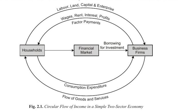
In the two-sector economy there are only households and firms. Households supply resources (land, labour, capital, enterprise) to firms and receive factor payments (wages, rent, interest, profits). Households then spend that income on goods and services produced by firms, so money flows back to firms as consumption expenditure. This is the circular flow of income, and it continues indefinitely.
Crucially, the volume of this flow is not constant: in years of depression the circular flow contracts, and in years of prosperity it expands, because the flow of money is a measure of national income.
2Saving, Investment and the Condition for a Constant Flow
If households save part of their income, their expenditure falls and the money flow to firms contracts; firms hire fewer workers and total income falls. Economists therefore call saving a leakage from the money expenditure flow p. 22.
But savings need not reduce aggregate spending if they find their way back into the expenditure flow. Households deposit savings with financial institutions (the financial market), and business firms borrow from that market for investment in capital goods. Investment is therefore an injection of money into the circular flow.
If planned investment falls short of planned saving, income, output and employment fall and the flow contracts; stocks pile up in shops, retailers order less, less is produced, fixed investment falls. If instead investment demand rises, income, output and employment increase and the flow expands p. 23.
Classical economists believed the rate of interest automatically coordinates saving and investment. Keynes refuted this: since investment is made by business enterprises and saving mostly by households, for different reasons, there is no guarantee planned investment equals planned saving — so fluctuations in income, output and employment are inevitable unless the government takes corrective steps.
3Three-Sector Model: Adding Government
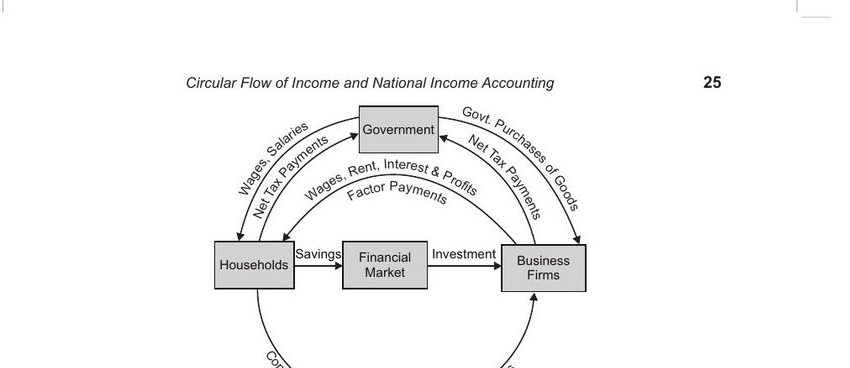
Adding government introduces two new flows: tax payments from households and firms to the government (net of transfer payments, which are treated as negative taxes), and government purchases of goods and services. Government may also finance spending by borrowing from the financial market, which increases demand for credit and raises the rate of interest — lowering private investment while encouraging households to save more p. 25.
The algebra of the three-sector model is a favourite exam target:
Equation (v) is very significant. If G > T the government has a budget deficit, financed by borrowing from the financial market — which requires private investment (I) to be less than household saving (S). Thus government borrowing crowds out private investment.
The textbook also splits national saving into two parts p. 26:
For the economy to remain in a steady state, the sum of private and public saving must equal investment.
4Four-Sector Model: Adding the Foreign Sector
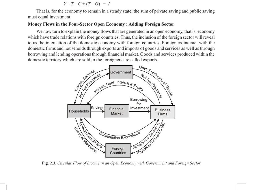
An open economy has trade relations with foreign countries. Goods and services produced within the domestic territory and sold to foreigners are exports (X); purchases of foreign-made goods by domestic households are imports (M). If exports equal imports there is a balance of trade; if X > M there is a trade surplus; if M > X, a trade deficit p. 27. Countries also interact through borrowing and lending in increasingly integrated world financial markets.
5Leakages and Injections
Pulling the models together gives the syllabus's "leakages in the circular flow model":
| Leakages (withdrawals) | Injections |
|---|---|
| Saving (S) — income not spent on consumption | Investment (I) — firms borrow and spend on capital goods |
| Taxes (T) — paid to government | Government expenditure (G) — purchases of goods and services |
| Imports (M) — spending that goes abroad | Exports (X) — foreign spending on domestic output |
Consequence of leakages exceeding injections: the flow of income contracts — output, employment and income fall. When injections exceed leakages, the flow expands.
6Exam-Ready Answer
In a modern monetary economy, money acts as a medium of exchange, so corresponding to the real flows of resources, goods and services there are flows of money, each money flow being in the opposite direction to the real flow. In the simple two-sector model, households supply economic resources such as land, labour and capital to business firms and receive factor payments in the form of wages, rent, interest and profits; households then spend this income on the goods and services produced by firms, so money flows back to the firms as consumption expenditure. This constitutes the circular flow of income, whose volume contracts in years of depression and expands in years of prosperity. When households save a part of their income, expenditure on goods declines and the money flow to firms contracts, so saving is a leakage from the expenditure flow; however, savings deposited in the financial market are borrowed by firms for investment in capital goods, so investment is an injection. For the circular flow to continue at a constant level, planned saving must equal planned investment. In the three-sector model the government is added, introducing tax payments as a leakage and government purchases as an injection; since total expenditure C + I + G must equal total income C + S + T, it follows that I + G = S + T, and rearranging gives G − T = S − I, which shows that when the government runs a budget deficit it must borrow from the financial market, so that private investment falls short of saving — that is, government borrowing crowds out private investment. In the four-sector or open-economy model, exports are an injection and imports a leakage, and the flow remains constant when S + T + M = I + G + X. If total leakages exceed total injections, the circular flow of income contracts and output, employment and income fall; if injections exceed leakages, the flow expands.
7Possible Exam Questions
- Explain the circular flow of income in a two-sector economy with a diagram.
- Explain the circular flow model in a three-sector and four-sector economy.
- What are leakages and injections in the circular flow model? What are the consequences of leakages?
- Show that G − T = S − I. What does this equation imply about government borrowing?
- Why are planned saving and planned investment often unequal, though actual saving always equals actual investment?
8Common Mistakes
- Confusing planned with actual saving/investment. Planned values can differ (that's what causes fluctuations); actual values are identical by accounting definition.
- Putting imports on the injection side. Imports are a leakage; exports are the injection.
- Drawing the two-sector diagram with only one loop — you need both the real flow and the money flow, in opposite directions.
- ENCircular Flow of Income: Simple Explanation of 2, 3 & 4 Sector ModelsPM Expert
- HI/ENCircular flow of Income in two, three and four Sector EconomyMini Sethi
- ENCircular Flow in a Three-Sector EconomyMagnet Brains
- ENCircular Flow in a Four-Sector EconomyMagnet Brains
2. Concepts of National Income Core syllabus concept
1Understand the Concept
National income can be looked at in three equivalent ways p. 21: (a) the sum of values of all final goods and services produced; (b) the sum of all incomes accruing to factors of production in a year; and (c) the sum of consumers' expenditure, net investment expenditure and government expenditure. All three give the same total, but each reflects one of the three basic activities of the economy — production, distribution and expenditure.
The textbook is emphatic that national product = national income, quoting J.R. Hicks: "The value of the net social product of the community and the sum of the incomes of its members are exactly equal." This holds exactly in the simple two-sector case; in a real economy it holds after allowing for depreciation and net indirect taxes p. 29.
| Concept | Definition | Formula |
|---|---|---|
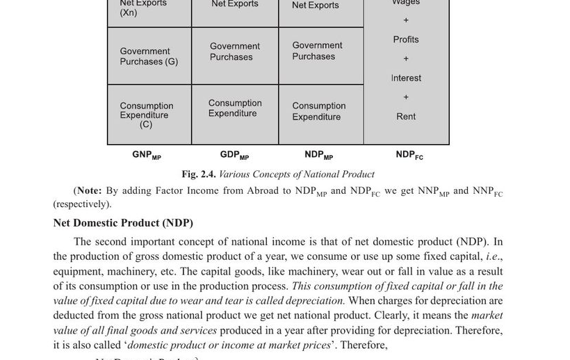
| GDP Gross Domestic Product | The total market value of all final goods and services produced in a year in the domestic territory of a country. A monetary measure; only final goods counted, to avoid double counting. | GDP = C + I + G + NX where NX = X − M |
| GNP Gross National Product | GDP plus net factor income from abroad. GDP is territory-based; GNP is resident-based. | GNPMP = GDPMP + Net factor income from abroad |
| NDP Net Domestic Product | GDP minus depreciation (consumption of fixed capital — the fall in value of capital goods due to wear and tear). | NDP = GDP − Depreciation |
| NNP Net National Product | GNP minus depreciation. NNP at factor cost is National Income. | NNPFC = NNPMP − Net indirect taxes |
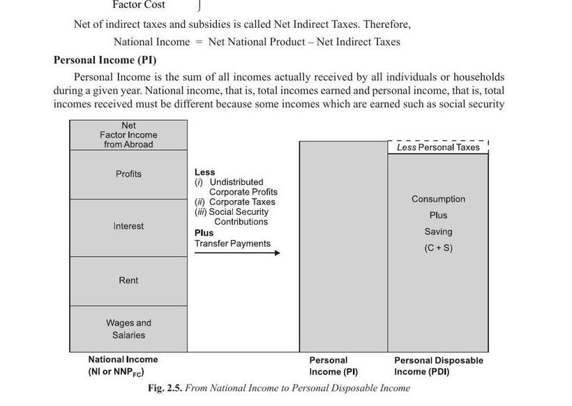
| PI Personal Income | Income actually received by households, as against income earned. | PI = NI − Social Security Contributions − Corporate Income Taxes − Undistributed Corporate Profits + Transfer Payments |
| PDI Personal Disposable Income | What remains of personal income after personal taxes. Can only be consumed or saved. | PDI = PI − Personal Taxes PDI = Consumption + Saving |
2Key Distinctions
- Final vs intermediate goods. Final goods are purchased for final use, not for resale or further processing. Intermediate goods are excluded because the value of final goods already includes them — including both would be double counting. The textbook's example: raw cotton worth ₹1,000 and cotton cloth worth ₹2,000 — adding both double-counts the cotton p. 30.
- Only current production counts. GNP is a flow measure per time period. Transactions in old houses, cars or factories built earlier, and purchases/sales of stocks and bonds, are excluded because they do not involve current production.
- Net factor income from abroad = factor income received from abroad by normal residents − factor income paid to foreign residents for services rendered within the domestic territory. Its three components are: net compensation to employees; net income from property (rent, interest, profits/dividends); and net retained earnings of resident companies abroad p. 31.
- Do not confuse net factor income from abroad with net exports. Net exports are part of both GDP and GNP; net factor income from abroad is what distinguishes GNP from GDP.
- Nominal vs Real GNP. Nominal GNP uses current-year prices; real GNP values current output at base-year prices. Real GNP is used to measure economic growth and compare living standards p. 43.
3Exam-Ready Answer
Gross Domestic Product is defined as the total market value of all final goods and services produced in a year within the domestic territory of a country. It is a monetary measure, and for it to be calculated accurately all goods and services produced in a year must be counted once and only once: only final goods, which are purchased for final use rather than for resale or further processing, are included, while intermediate goods are excluded because the value of final goods already includes them and counting both would involve double counting. GDP is obtained as consumption plus investment plus government purchases plus net exports, where net exports equal exports minus imports. Gross National Product is the money value of all final goods and services produced together with net factor income earned from abroad, so that GNP at market prices equals GDP at market prices plus net factor income from abroad; net factor income from abroad is the difference between factor income received from abroad by normal residents and factor income paid to foreign residents for services rendered within the domestic territory. When depreciation, that is the consumption of fixed capital due to wear and tear, is deducted from the gross measures, we obtain Net Domestic Product and Net National Product respectively, and Net National Product at factor cost is what is called National Income. Personal income is the income actually received by households, obtained from national income by subtracting social security contributions, corporate income taxes and undistributed corporate profits, which are earned but not received, and adding transfer payments, which are received but not currently earned. Personal disposable income is personal income minus personal taxes, and can either be consumed or saved. Finally, nominal GNP measures output at current prices while real GNP values current output at base-year prices, and the ratio of nominal to real GNP multiplied by 100 gives the GNP deflator, which measures the rate of inflation.
4Possible Exam Questions
- Define GDP, GNP, NDP and NNP. Distinguish between them.
- Differentiate between GDP and GNP. What is net factor income from abroad?
- What are final and intermediate goods? Why are intermediate goods excluded from national income?
- How is personal disposable income derived from national income?
- Distinguish between nominal and real GNP. What is the GNP deflator?
5Common Mistakes
- Confusing net factor income from abroad (GDP → GNP) with net exports (already inside GDP).
- Forgetting that National Income specifically means NNP at factor cost, not NNP at market price.
- Including second-hand sales or share transactions in GNP — they are not current production.
- HI/ENNational Income Concepts — GDP, GNP, NNP, NDPMini Sethi
- HINational Income — GDP/GNP/NNP/NDP (Hindi)E.Z. Classes
- ENNational Income — GDP GNP NDP NNP Explained (Indian Economy)StudyIQ IAS
3. Measurement of National Income & Its Limitations Core syllabus concept
1Understand the Concept
Since factor incomes arise from the production of goods and services, and incomes are spent on goods and services produced, three alternative methods of measuring national income are possible p. 34.
2The Three Methods
(1) Value Added Method (also called the output or production method). The economy is divided into industrial sectors — agriculture, fishing, mining, construction, manufacturing, trade, transport, communication, services — and the net value added at factor cost by each enterprise and sector is estimated:
The great advantage of this method is that it reveals the relative importance of the different sectors of the economy by showing their respective contributions to national income.
Precautions in the value added method p. 35: include imputed rent of self-occupied houses; exclude sale/purchase of second-hand goods (but include the commission or brokerage earned on them, since that is a current service); include production for self-consumption valued at market prices; exclude the value of services of housewives.
(2) Income Method. National income is measured as the sum of factor incomes — compensation of employees, rent, interest and profits — generated in production p. 37.
(3) Expenditure Method. National income is measured as the sum of final expenditures: private final consumption expenditure, government final consumption expenditure, gross domestic capital formation (investment) and net exports p. 39.
3Limitations of GDP as a Measure of Social Welfare
National income has often been used as a measure of economic welfare, but modern economists doubt its validity. To obtain a true measure — called Net Economic Welfare (NEW) — adjustments must be made in both directions pp. 43–44:
| Ought to be ADDED | Ought to be DEDUCTED |
|---|---|
|
Value of leisure. GNP attaches no significance to leisure, yet people derive satisfaction from it. If average working hours fall, national income may fall but welfare may rise. Non-marketed personal services. Services of housewives to family members, or personal services such as gardening or painting one's own house, greatly raise welfare but are not recorded. |
Environmental pollution. Modern industry pollutes air, water and calmness, significantly reducing welfare. These are the "costs of economic growth" and should be assigned negative values. "Regrettable costs." Wasteful and non-productive expenditure such as government spending on police, law courts and defence — regrettable necessities that do not increase welfare. |
Other standard difficulties in measuring national income include the risk of double counting, the problem of valuing non-monetised transactions and production for self-consumption, the existence of the unreported/black economy, and the inadequacy and unreliability of statistical data, particularly in developing countries.
4Uses of National Income Data
Your syllabus names this topic explicitly — "National Income: Concepts and Measurement, Uses and Limitations in Measuring National Income" — and the lecture deck gives the list Slide 14. If a question asks why we bother measuring national income at all, this is the answer:
| Use | What it lets you do |
|---|---|
| Standard of living comparison | Compare living standards between countries, usually via per capita income. |
| Economic performance over time | Judge whether the economy is growing, stagnating or contracting, by comparing real national income across years. |
| National planning | Set targets and allocate resources — planning is impossible without knowing the size of the pie. |
| Sectoral contribution | See how much agriculture, industry and services each contribute, and how that mix is shifting. This is the value-added method's special strength. |
| Economic policy | Provide the evidence base for fiscal and monetary decisions — you cannot close an output gap you have not measured. |
| National expenditure | Show how the nation's income is split between consumption and investment, which determines future growth. |
| Public sector | Assess the size and role of government in the economy. |
| Distribution of income | Study how income is shared between factors and between groups, which is the starting point for any question about inequality. |
Related concept from the same deck: per capita income is the average income of the people of a country in a particular year — national income divided by population Slide 7. It is the figure normally used for standard-of-living comparisons, precisely because total national income says nothing about how many people have to share it.
5Difficulties in Measurement — general, and specific to each method
The lecture deck separates the difficulties that affect every method from those that are a weakness of one particular method. That structure is worth copying in an answer, because it shows you know why three methods exist.
General difficulties Slide 15:
- Non-monetised transactions. Goods and services exchanged without a money payment — services rendered out of love, courtesy or kindness — have no price to record.
- The unorganised sector. Its contribution goes largely unrecorded, and the income of those who do not pay income tax is very hard to identify.
- Multiple sources of earnings / multi-occupations. Part-time activity commonly goes unrecognised, so that income never enters the estimate.
- Categorisation of goods and services, and double counting. Whether a given item is final or intermediate is often not clear-cut, and getting it wrong inflates the total.
Method-specific limitations:
| Method | Its own weakness |
|---|---|
| Product / output Slide 13 | Double counting, because the line between a final and an intermediate product is unclear; hard to apply to the tertiary sector, since it needs output measurable in physical terms; excludes non-marketed products (the outcome of a hobby) and output the producer consumes himself. |
| Income Slide 10 | Excludes non-monetary income — a farmer and family working their own field contribute output but record no income; excludes non-marketed services whose money value is difficult to ascertain, the standard example being a mother's services to her family. |
| Expenditure Slide 11 | Ignores the barter system; ignores own consumption; and is affected by inflation, so nominal expenditure can rise while real output does not. |
Notice the pattern: every method misses roughly the same real activity — unpaid work, self-consumption, and the informal economy — but each misses it for a different reason. That single sentence is a strong way to close an answer on this topic.
6Exam-Ready Answer
Since factor incomes arise from the production of goods and services and incomes are spent on the goods and services produced, three alternative methods of measuring national income are possible. The value added or production method divides the economy into industrial sectors and estimates the net value added at factor cost by each enterprise and sector: the value of output equals sales plus change in stocks, gross value added at market prices is obtained by deducting intermediate consumption from the value of output, net value added at market prices is obtained by deducting depreciation, and net value added at factor cost by further deducting net indirect taxes; summing across sectors gives net domestic product at factor cost, to which net factor income from abroad is added to obtain national income. The great advantage of this method is that it reveals the relative importance of the different sectors of the economy. Certain precautions are necessary: the imputed rent of self-occupied houses must be included, the sale and purchase of second-hand goods excluded though the commission earned on them included, production for self-consumption valued at market prices and included, and the services of housewives excluded. The income method measures national income as the sum of factor incomes — compensation of employees, rent, interest and profits — while the expenditure method measures it as the sum of private final consumption expenditure, government final consumption expenditure, gross domestic capital formation and net exports. National income is, however, an imperfect measure of economic welfare. To arrive at a truer measure, often called Net Economic Welfare, the value of leisure and of non-marketed personal services such as those rendered by housewives ought to be added, while the costs of environmental pollution caused by production and regrettable costs such as expenditure on police, law courts and defence ought to be deducted. Further difficulties in measurement include the danger of double counting, the valuation of non-monetised transactions and production for self-consumption, the existence of an unreported economy, and the unreliability of statistical data in developing countries.
Despite these limitations, national income data are indispensable. They are used to compare standards of living between countries, to judge economic performance over time, for national planning, to measure the sectoral contribution of agriculture, industry and services, to frame economic policy, to examine the composition of national expenditure between consumption and investment, to assess the size of the public sector, and to study the distribution of income. The practical difficulties of estimation include non-monetised transactions such as services rendered out of love or kindness, the unrecorded contribution of the unorganised sector, part-time and multiple occupations whose earnings go unrecognised, and the categorisation of goods which gives rise to double counting. Each method also has a weakness of its own: the product method suffers from double counting and cannot easily be applied to the tertiary sector; the income method omits non-monetary income such as that of a farmer working his own field and non-marketed services such as those of a mother to her family; and the expenditure method ignores barter and own consumption and is distorted by inflation.
7Possible Exam Questions
- Explain the three methods of measuring national income.
- Explain the value added method. What precautions should be taken while using it?
- Discuss the limitations of GDP as a measure of social welfare.
- What are the difficulties in measuring national income in a developing country like India?
- What is Net Economic Welfare? What items should be added to and deducted from national income to obtain it?
- State the uses of national income data.
- Explain the limitations of the income method and of the product method of measuring national income.
8Common Mistakes
- Excluding both second-hand goods and the brokerage on them. The commission is included — it is a current service.
- Forgetting that services of housewives are excluded from national income but should be added back when constructing Net Economic Welfare.
- Listing methods without the value-added chain (Value of output → GVAMP → NVAMP → NVAFC), which is where the marks are.
- ENThree ways to calculate National Income — Product, Expenditure & Income methodsEasy Learning Economics
- HI/ENNational Income Concepts & Measurement (UGC NET / JRF Macro)Mini Sethi
4. Consumption Function Core syllabus concept
1Understand the Concept
Just as the demand for a good depends on its price, consumption of a community depends on the level of income — consumption is a function of income. The consumption function is the whole schedule which describes the amounts of consumption at various levels of income, and must be carefully distinguished from the amount of consumption at one specific income level p. 149.
The central fact Keynes emphasised: when income rises, consumption also rises, but not by as much as income — because part of the increment in income is saved.
where a is the intercept (autonomous consumption), b is the slope — the marginal propensity to consume — and Y is current income.
| Concept | Definition | Formula |
|---|---|---|
| APC — Average Propensity to Consume | The proportion of income that is consumed. | APC = C / Y |
| MPC — Marginal Propensity to Consume | The change in consumption caused by a change in income; the slope of the consumption function. | MPC = ΔC / ΔY |
Two features of the Keynesian consumption function are exam-critical p. 150:
- MPC remains constant (the function is linear) while APC falls as income increases. In the textbook's Table 6.1, MPC stays at 0.70 throughout while APC falls from 0.950 to 0.856.
- Therefore MPC < APC at all income levels, and the increase in consumption is not proportional to the increase in income.
- MPC lies between zero and unity (0 < MPC < 1). If MPC were 0 the whole increment would be saved and the curve horizontal; if MPC were 1 the whole increment would be consumed and the curve would coincide with the 45° line p. 155.
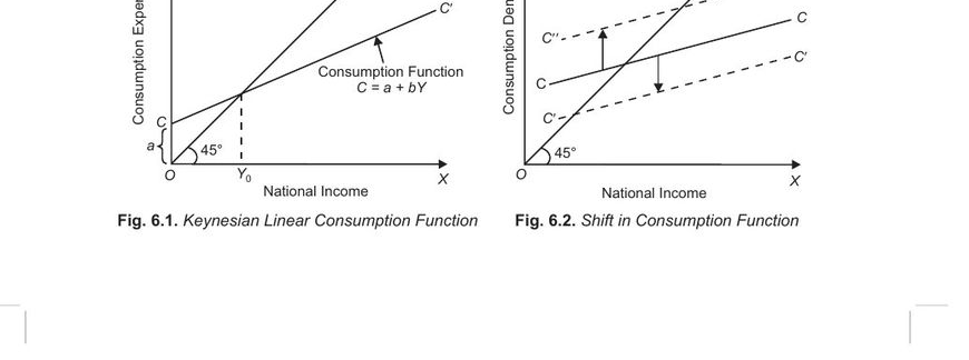
Reading the diagram. The 45° line OZ is drawn so that every point on it is equidistant from both axes — if the consumption curve coincided with it, consumption would equal income at every level. In practice the consumption curve CC′ deviates from it: at low income levels CC′ lies above OZ (consumption exceeds income — the nation draws on accumulated savings or borrows); at income OY₀ consumption equals income (the break-even point); beyond that CC′ lies below OZ and the gap — which is saving — widens as income rises p. 151.
2Simple Explanation
3Worked Example
| Income Y (₹ cr) | Consumption C (₹ cr) | APC = C/Y | MPC = ΔC/ΔY |
|---|---|---|---|
| 1000 | 950 | 0.950 | — |
| 1100 | 1020 | 0.927 | 70/100 = 0.70 |
| 1200 | 1090 | 0.908 | 0.70 |
| 1300 | 1160 | 0.892 | 0.70 |
| 1500 | 1300 | 0.867 | 0.70 |
| 1600 | 1370 | 0.856 | 0.70 |
Income rises by ₹100 crore each step; consumption rises by ₹70 crore and ₹30 crore is saved. MPC constant at 0.70; APC falling throughout; MPC < APC at every level.
4Exam-Ready Answer
The consumption function relates the amount of consumption to the level of income, and is the whole schedule which shows the amounts of consumption at various levels of income; it must be distinguished from the amount of consumption, which is the amount consumed at one specific level of income. Keynes emphasised that when income rises, consumption also rises but not by as much as income, because a part of the increment in income is saved. Since Keynes was concerned with the short run, he assumed the price level, rate of interest and stock of wealth to be constant, so that consumption is a function of current income, written as C = f(Y), and in its specific linear form as C = a + bY, where a is the intercept term representing autonomous consumption, b is the slope of the function representing the marginal propensity to consume, and Y is current income. The average propensity to consume is the proportion of income that is consumed, C divided by Y, while the marginal propensity to consume is the ratio of the change in consumption to the change in income and is given by the slope of the consumption function curve. In the Keynesian consumption function the marginal propensity to consume remains constant while the average propensity to consume falls as income increases, which implies that the increase in consumption is not proportional to the increase in income; consequently the marginal propensity to consume is less than the average propensity to consume at all levels of income. The marginal propensity to consume is neither zero nor equal to one but varies between zero and unity, for if it were zero the whole increment in income would be saved and the consumption curve would be horizontal, while if it were unity the whole increment would be consumed and the curve would coincide with the 45° line. Diagrammatically, at low levels of income the consumption function curve lies above the 45° line because consumption exceeds income, at one level of income it intersects the 45° line where consumption equals income, and beyond that it lies below the 45° line with the widening gap between income and consumption representing saving.
5Possible Exam Questions
- What is the consumption function? Explain the Keynesian consumption function with a diagram.
- Distinguish between average propensity to consume and marginal propensity to consume.
- Why is MPC always between zero and one?
- Given a consumption schedule, calculate APC and MPC at each income level.
- Explain why APC falls while MPC remains constant in the Keynesian consumption function.
6Common Mistakes
- Swapping APC and MPC. APC uses total C and Y; MPC uses the changes ΔC and ΔY.
- Saying both APC and MPC fall. In the linear Keynesian function MPC is constant; only APC falls.
- Forgetting the 45° line when drawing the diagram — without it you cannot show the break-even point or the saving gap.
- HI/ENConsumption Function — Propensity to Consume, APC, MPC, APS, MPSMini Sethi
- ENConsumption and Saving Function | Keynes' Law of Consumption | MPC | MPSEasy Learning Economics
- HIConsumption Function & Saving Function (APC & MPC)STUDY 24 Udaipur
5. Saving Function and Investment Function Core syllabus concept
1Understand the Concept
Saving is defined as the part of income which is not consumed, since disposable income is either consumed or saved p. 155:
The saving function is the counterpart of the consumption function — given a consumption function, the corresponding saving function can be derived. Taking the Keynesian form C = a + bY:
where (1 − b) is the marginal propensity to save (MPS).
Given C = 150 + 0.80Y:
S = Y − 150 − 0.80Y = −150 + 0.20Y
Here 0.20 is the marginal propensity to save. Note that MPC + MPS = 0.80 + 0.20 = 1.
| Concept | Definition | Formula |
|---|---|---|
| APS — Average Propensity to Save | The proportion of disposable income that is saved. | APS = S / Y |
| MPS — Marginal Propensity to Save | The change in saving caused by a change in income. | MPS = ΔS / ΔY = 1 − MPC |
The key relationship, derived by dividing C + S = Y through by Y:
So if a society consumes 75% of its disposable income (APC = 0.75), it saves 25% (APS = 0.25). And since APC falls as income increases, APS rises as income increases p. 156.
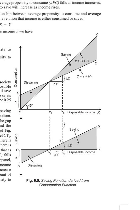
The saving curve SS in the lower panel measures the gap between the consumption curve CC and the income line OZ in the upper panel. Up to income level OY₁ consumption exceeds income — there is dissaving (the curve lies below the horizontal axis). Beyond OY₁ there is positive saving, and as income rises both the absolute amount of saving and the average propensity to save increase.
2The Investment Function
Investment is the other component of aggregate demand. In the Keynesian framework, investment depends on the rate of interest together with the marginal efficiency of capital (MEC) — the expected rate of profit from an investment project. Since a lower rate of interest makes borrowing cheaper, investment varies inversely with the rate of interest, giving a downward-sloping investment demand curve. This inverse relationship is precisely what is used to derive the IS curve in the next concept p. 297.
Keynes attributed business cycles largely to the volatility of investment: a sudden collapse of the expected rate of profit (the marginal efficiency of capital), caused by adverse changes in entrepreneurs' expectations, lowers investment and causes a downswing p. 587.
3Exam-Ready Answer
Saving is defined as that part of income which is not consumed, since disposable income is either consumed or saved, so that Y equals C plus S and therefore S equals Y minus C. Like consumption, saving is a function of income, written as S = f(Y), and the saving function is the counterpart of the consumption function, so that given a particular consumption function the corresponding saving function can be derived. Taking the Keynesian consumption function C = a + bY and substituting it into S = Y − C gives S = −a + (1 − b)Y, where (1 − b) is the marginal propensity to save and b is the marginal propensity to consume. For example, if the consumption function is C = 150 + 0.80Y, then the saving function is S = −150 + 0.20Y, where 0.20 is the marginal propensity to save; it follows that the sum of the marginal propensity to consume and the marginal propensity to save is equal to one. The average propensity to save is the proportion of disposable income that is saved, S divided by Y, and dividing the identity C + S = Y throughout by Y gives APC + APS = 1, or APS = 1 − APC; thus if a society consumes 75 per cent of its disposable income its average propensity to save is 25 per cent. Since the average propensity to consume falls as income increases, the average propensity to save rises as income increases. Diagrammatically, the saving curve measures the gap between the consumption curve and the 45° income line: up to the break-even level of income consumption exceeds income and there is dissaving, so the saving curve lies below the horizontal axis, while beyond that level saving is positive and both the absolute amount of saving and the average propensity to save increase with income. Investment, the other component of aggregate demand, is determined by the rate of interest together with the marginal efficiency of capital, and varies inversely with the rate of interest.
4Possible Exam Questions
- What is the saving function? Derive the saving function from a given consumption function.
- Given C = 150 + 0.80Y, derive the saving function and state the MPS.
- Prove that APC + APS = 1 and that MPC + MPS = 1.
- What is dissaving? Show it on a diagram.
- Explain the investment function. On what does investment depend?
5Common Mistakes
- Sign error when deriving S: the intercept becomes negative (−a), which is what produces dissaving at low incomes.
- Writing MPS = 1 − APC. It is MPS = 1 − MPC; the average-pair relation is APS = 1 − APC.
- Omitting the marginal efficiency of capital when asked what determines investment.
6. Keynesian Model: Aggregate Demand and Aggregate Supply Core syllabus concept
1Understand the Concept
Keynes, concerned with an economy gripped by depression, assumed the price level remained constant. Classical economists, by contrast, held that output was determined by real factors and was unaffected by the general price level, which was determined by the quantity of money — the classical dichotomy. The AD-AS model with a flexible price level highlights the breakdown of that dichotomy and is used to explain fluctuations in output, price level and inflation p. 230.
Aggregate Demand (AD) is the total desired quantity of goods and services bought by consumer households, private investors, government and foreigners at each possible price level, other things held constant. It is not a quantity demanded at one price but a whole schedule, represented by a curve. Its four components are consumption demand, private investment demand, government purchases, and net exports.
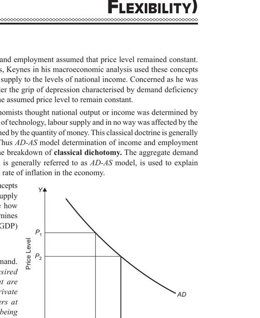
Why the AD curve slopes downward. A rise in the price level reduces aggregate demand through three effects p. 238:
- Wealth (real balance) effect — much wealth is held as bank deposits, bonds and shares; a higher price level reduces the real purchasing power of that wealth, inducing people to spend less, so consumption falls.
- Interest rate effect — a higher price level reduces the supply of real money balances (Mˢ/P), shifting the money supply curve left; given money demand, the rate of interest rises, which induces private investment to decline.
- Net exports effect — a higher domestic price level adversely affects the country's exports, causing net exports to fall.
Aggregate Supply (AS) is the total output of goods and services that firms want to produce at each possible price level — again a whole schedule, represented by a curve p. 238. There is considerable disagreement about its shape:
| View | Shape of AS curve | Reasoning |
|---|---|---|
| Classical | Vertical at full-employment output | Full employment of resources normally prevails; output is determined by real factors, so a change in price level cannot change output. |
| Keynes | Horizontal up to full employment, then vertical | With excess capacity and unemployed resources in depression, output can expand without any rise in the price level until full employment is reached. |
| Short-run (SAS) | Upward-sloping | In the short run, money wages are sticky, so a higher price level raises profit margins and induces firms to produce more. |
| Long-run (LAS) | Vertical at potential GDP | In the long run wages and prices fully adjust, so output returns to its potential level regardless of the price level. |
Multiplier with a flexible price level. With an upward-sloping SAS curve, an increase in autonomous expenditure works in two stages: first the AD curve shifts right, raising GNP at the given price level; second, because SAS slopes upward, the price level rises, which claws back part of that increase. So the multiplier effect on real GDP is still positive but smaller than it would be if the price level were fixed — and the steeper the SAS curve, the greater the rise in price level and the smaller the multiplier effect p. 238.
2Simple Explanation
3Exam-Ready Answer
Aggregate demand is the total desired quantity of goods and services that are bought by consumer households, private investors, government and foreigners at each possible price level, other things being held constant. It is therefore not any quantity demanded at a particular price level but a whole schedule of total output demanded at various price levels, represented by a curve, and it has four components: consumption demand, private investment demand, government purchases of goods and services, and net exports. The aggregate demand curve slopes downward for three reasons. First, through the wealth or real balance effect: since much wealth is held in the form of bank deposits, bonds and shares, a rise in the price level reduces the real purchasing power of that wealth and induces people to spend less, so consumption expenditure declines. Second, through the interest rate effect: a rise in the price level reduces the supply of real money balances, which causes the rate of interest to rise and induces private investment expenditure to decline. Third, through the net exports effect: a rise in the domestic price level adversely affects the country's exports, causing net exports to fall. Aggregate supply is the total output of goods and services that firms want to produce at each possible price level, and is likewise a whole schedule represented by an aggregate supply curve. There is disagreement about its shape: classical economists, assuming that full employment of resources normally prevails, drew it as vertical at the full-employment level of output, so that changes in the price level cannot affect output; Keynes, concerned with an economy having excess capacity and unemployed resources, drew it as horizontal up to full employment, so that output could expand without any rise in the price level; the short-run aggregate supply curve slopes upward because money wages are sticky in the short run; and the long-run aggregate supply curve is vertical at potential GDP because wages and prices adjust fully in the long run. Because the short-run aggregate supply curve slopes upward, an increase in autonomous expenditure raises the price level as well as output, so the multiplier effect on real GDP is smaller than it would be if the price level remained fixed, and the steeper the short-run aggregate supply curve, the greater the rise in the price level and the smaller the multiplier effect.
4Possible Exam Questions
- What is aggregate demand? Why does the aggregate demand curve slope downward?
- Explain the shape of the aggregate supply curve according to the classical economists and according to Keynes.
- Explain the determination of equilibrium output and price level using the AD-AS model.
- How does a flexible price level affect the size of the multiplier?
- Distinguish between the short-run and long-run aggregate supply curves.
5Common Mistakes
- Explaining the downward-sloping AD curve using the microeconomic law of demand (substitution/income effects). At the macro level the reasons are the wealth, interest-rate and net-export effects.
- Drawing the Keynesian AS curve as upward-sloping throughout — Keynes' own version is horizontal until full employment, then vertical.
- Forgetting that the classical vertical AS is drawn at the full-employment level of output.
- ENLearn the AD-AS Model in 6 MinutesIn Case of Econ Struggles
- ENKeynesian Aggregate Supply / Aggregate Demand (AS/AD)EconplusDal
- ENThe AD-AS Model Explained | Foundations of MacroeconomicsMacro Economics with Michael
7. Goods and Money Market: The IS-LM Model Core syllabus concept
1Understand the Concept — Why the model exists
In Keynes' simple model, national income is determined by goods market equilibrium, while the rate of interest is determined by money market equilibrium. Changes in the interest rate affect investment and hence income. But critics pointed out an apparent flaw: there seemed to be no reverse influence of changes in the goods market back on the money market p. 297.
J.R. Hicks and others showed that the level of income — which depends on investment and consumption demand — determines the transactions demand for money, which in turn affects the rate of interest. Hicks, Hansen, Lerner and Johnson therefore put forward an integrated model in which investment, national income, the rate of interest and the demand for and supply of money are mutually interdependent, represented by two curves — IS and LM. This model shows how national income and the rate of interest are jointly determined by simultaneous equilibrium in the two interdependent markets, and it has become a standard tool for discussing monetary and fiscal policy.
The four building blocks. Your lecture deck lists exactly what the model is assembled from Slide 9 — worth stating in an opening paragraph, because it shows the model is not new theory but a synthesis of things you already know:
- The investment demand function — investment as a function of the rate of interest.
- The consumption function — C = a + bY, from Concept 4 above.
- The money demand function — liquidity preference, Md = L(Y, r).
- The quantity of money — the money supply, fixed by the central bank.
As the deck puts it, the IS-LM model succeeded in integrating the theory of money with the theory of income determination, so that we can trace the effect of a change in income, money supply, investment or money demand on both the rate of interest and the level of income at once. Note the direction of causation the deck stresses at each stage: in the goods market, a fall in the rate of interest lowers the cost of investment projects and thereby raises their profitability, so businessmen undertake greater investment, and the lower the rate of interest the higher the equilibrium level of national income Slide 4. In the money market, the LM curve by itself determines neither national income nor the interest rate — it only states the combinations of the two at which the money market is in equilibrium Slide 7. That is exactly why you need both curves.
2The IS Curve — Goods Market Equilibrium
The goods market is in equilibrium when aggregate demand equals income. Introducing the rate of interest as a determinant of investment makes investment an endogenous variable: when the rate of interest falls, investment increases, which raises aggregate demand and therefore the equilibrium level of income p. 297. Plotting each rate of interest against the income level it produces gives the IS curve, which slopes downward to the right.
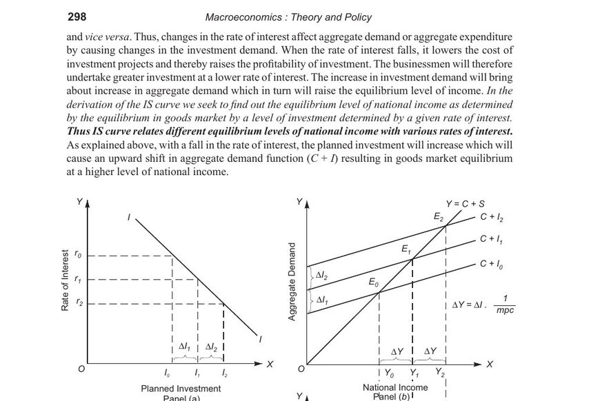
Shifts in the IS curve. The IS curve shifts right when government expenditure or autonomous investment increases, or when autonomous consumption increases due to a cut in personal income tax; the size of the shift equals the change in the variable times the relevant multiplier. For a tax cut, the rightward shift equals ΔT × [MPC / (1 − MPC)], where MPC/(1−MPC) is the tax multiplier. It shifts left for the reverse changes p. 301.
3The LM Curve — Money Market Equilibrium
According to Keynes, demand for money to hold depends on the transactions motive and the speculative motive. Money held for transactions is a function of income; the demand for money also depends on the rate of interest, which is the cost of holding money, since by holding money rather than lending it one forgoes interest p. 301:
Higher income means a higher money demand curve; with a fixed money supply, money market equilibrium then requires a higher rate of interest. Plotting these income–interest combinations gives the LM curve, which slopes upward to the right.
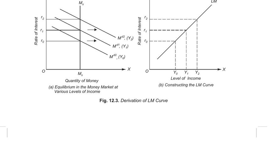
Shifts in the LM curve p. 303: an increase in real money supply (M/P) shifts LM to the right; a decrease shifts it up and to the left. An increase in the money demand function (liquidity preference) for a given income raises the interest rate and shifts LM up and to the left; a decrease shifts it down and to the right.
4Simultaneous Equilibrium
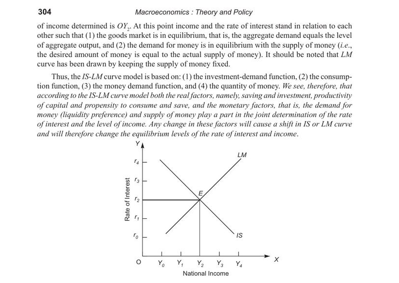
The point where IS and LM intersect gives the equilibrium rate of interest and the equilibrium level of national income simultaneously — the goods market and money market are both in equilibrium only at that combination.
5Using IS-LM for Policy
| Policy | Effect on curves | Result |
|---|---|---|
| Expansionary fiscal policy (↑ G or ↓ T) | IS shifts right | Income rises and the rate of interest rises. The rise in income is less than the full multiplier effect, because the higher interest rate crowds out some private investment p. 308. |
| Expansionary monetary policy (↑ money supply) | LM shifts right | Rate of interest falls and income rises p. 309. |
| Tight monetary policy (↓ money supply) | LM shifts left | Rate of interest rises and income falls. |
Elasticity of the LM curve and relative effectiveness of policy p. 312. The LM curve has three ranges: a near-horizontal Keynesian range at very low interest rates (the liquidity trap), an intermediate upward-sloping range, and a vertical classical range at high interest rates. In the horizontal (liquidity trap) range, monetary policy is ineffective while fiscal policy is fully effective; in the vertical classical range, monetary policy is highly effective while fiscal policy is completely crowded out.
6Exam-Ready Answer
In Keynes' simple model the level of national income is determined by equilibrium in the goods market, while the rate of interest is determined by equilibrium in the money market through the demand for and supply of money, so that changes in the rate of interest affect investment and hence income. It was objected, however, that there appeared to be no reverse influence of changes in the goods market on money market equilibrium. J. R. Hicks and others showed that the level of income, which depends on investment and consumption demand, determines the transactions demand for money and therefore affects the rate of interest. Hicks, Hansen, Lerner and Johnson accordingly put forward an integrated model in which investment, national income, the rate of interest and the demand for and supply of money are interrelated and mutually interdependent, represented by the IS and LM curves, which shows how the level of national income and the rate of interest are jointly determined by simultaneous equilibrium in the two interdependent markets. The IS curve is derived from goods market equilibrium, where aggregate demand equals income; since a fall in the rate of interest raises investment and therefore aggregate demand and equilibrium income, the IS curve slopes downward to the right. It shifts to the right when government expenditure or autonomous investment increases, or when autonomous consumption rises because of a cut in personal income taxes, the extent of the shift being the change in the variable multiplied by the relevant multiplier. The LM curve is derived from money market equilibrium; the demand for money depends on the transactions motive, which is a function of income, and on the rate of interest, which is the cost of holding money, so that demand for money may be written as Md = L(Y, r). A higher level of income raises the demand for money and, with a fixed money supply, requires a higher rate of interest for equilibrium, so the LM curve slopes upward to the right; it shifts rightward when the real money supply increases and leftward when it decreases or when liquidity preference increases. The point of intersection of the IS and LM curves determines the equilibrium rate of interest and the equilibrium level of national income simultaneously. The model is widely used for policy analysis: expansionary fiscal policy shifts the IS curve rightward, raising both income and the rate of interest, though the rise in income is less than the full multiplier effect because the higher interest rate crowds out some private investment, while expansionary monetary policy shifts the LM curve rightward, lowering the rate of interest and raising income.
7Possible Exam Questions
- Derive the IS curve. Why does it slope downward?
- Derive the LM curve. Why does it slope upward?
- Explain how the IS-LM model determines the rate of interest and national income simultaneously.
- Using the IS-LM model, explain the effect of an expansionary fiscal policy. Why is the rise in income less than the full multiplier effect?
- What causes the IS curve and the LM curve to shift?
- Explain the three ranges of the LM curve and the relative effectiveness of monetary and fiscal policy in each.
8Common Mistakes
- Getting the slopes the wrong way round. IS slopes downward (lower r → more I → higher Y); LM slopes upward (higher Y → more money demand → higher r).
- Saying fiscal expansion leaves the interest rate unchanged. In IS-LM it rises, and that is exactly what produces crowding out.
- Confusing a movement along a curve with a shift of it — G, T and autonomous investment shift IS; money supply and liquidity preference shift LM.
- ENIS-LM Model Explained | Full Concept & DerivationECOHOLICS
- HI/ENIS-LM Model | Its Derivation | Money Market & Goods Market EquilibriumMini Sethi
- ENIntermediate Macroeconomics 5/8: The IS-LM ModelScott W. Hegerty
- ENIS-LM Model — Definition, Diagram & Mathematical (complete)Economics Portal