Unit 08 — Inventory Control Models
The core "how much to order" models: EOQ, EBQ, and quantity discounts — fully worked, from your syllabus onward.
1. Economic Order Quantity (EOQ) Core syllabus concept
1Concept — What Is It Solving?
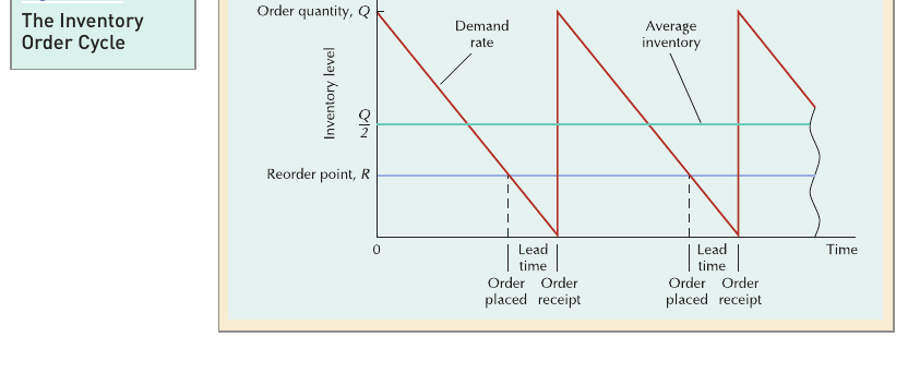
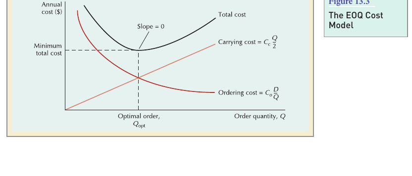
From Unit 7 you know carrying cost and ordering cost move in opposite directions as order size changes. The Economic Order Quantity (EOQ) model — the most widely used inventory model, first derived by Ford Harris in 1915 — finds the exact order size that minimises the sum of these two costs. It assumes: demand is known and constant, no shortages are allowed, lead time is constant, and the entire order quantity arrives at once (instantaneous receipt) — assumptions that make the model simple but still very robust in practice.
2Formula
3Variables
- D = annual demand (units/year)
- Co = ordering cost per order
- Cc = annual carrying cost per unit
- Q = order quantity; Qopt = the economic (optimal) order quantity
4When to Use It
Use the basic EOQ model whenever an item is replenished by ordering from an outside supplier (or a completed batch is received all at once), demand is reasonably steady, and you need to decide the order size that minimises total ordering + carrying cost.
5Step-by-Step Method
- Identify D (annual demand), Co (ordering cost), and Cc (annual carrying cost per unit).
- Compute Qopt = √(2·Co·D / Cc).
- Substitute Qopt back into TC = (CoD)/Q + (CcQ)/2 to find minimum total cost.
- If needed, compute number of orders/year = D/Qopt, and order cycle time = (working days/year) ÷ (D/Qopt).
6Textbook Example — Example 13.2
The ePaint Store has annual demand D = 10,000 gallons, ordering cost Co = $150/order, carrying cost Cc = $0.75/gallon/year.
Number of orders/year = 10,000/2,000 = 5; with 311 working days/year, order cycle time = 311/5 = 62.2 days between orders.
7Additional Example Illustrative example
A stationery store sells 4,800 units of a notebook per year, with an ordering cost of $20/order and a carrying cost of $2/unit/year.
Orders/year ≈ 4,800/310 ≈ 15.5, so the store reorders roughly every 3.4 weeks.
8Common Mistakes
- Using monthly figures for D but an annual rate for Cc (or vice versa) — all inputs must use the same time period, usually annual.
- Forgetting to take the square root at the final step.
- Computing TC using an arbitrary Q instead of the just-calculated Qopt.
- Not rounding Qopt to a sensible whole/practical unit in the final answer, where appropriate.
2. Economic Batch Quantity / Production Quantity Model (EBQ) Core syllabus concept
1Concept — What Is It Solving?
The basic EOQ model assumes the whole order arrives instantly. But when a company manufactures the item itself (rather than buying it from an outside supplier), the batch is produced gradually, at a finite production rate, while units are simultaneously being consumed/demanded — so inventory never actually reaches the full order quantity Q. The production quantity model (your syllabus calls this the Economic Batch Quantity, EBQ) relaxes the "instantaneous receipt" assumption to handle exactly this situation.
2Formula
3Variables
- d = daily demand rate; p = daily production rate (must have p ≥ d, otherwise no batch size works — output can't keep up with demand).
- All other variables (Co, Cc, D) same meaning as in basic EOQ.
4When to Use It
Use EBQ instead of basic EOQ whenever the item is produced in-house (not purchased ready-made) and produced gradually rather than delivered all at once — the classic case of a factory producing a component to feed its own assembly line, or a retailer that is also the manufacturer.
5Textbook Example — Example 13.3
ePaint now manufactures its own Ironcoat paint in-house: D = 10,000 gal/year, Co = $150 (setup cost), Cc = $0.75/gal, operating 311 days/year at production rate p = 150 gal/day, so d = 10,000/311 = 32.2 gal/day.
Production run = Q/p = 2,256.8/150 = 15.05 days; number of runs/year = D/Q = 10,000/2,256.8 ≈ 4.43 runs/year.
Maximum inventory level = Q(1 − d/p) = 2,256.8×(1 − 32.2/150) ≈ 1,772 gallons — this, not Q itself, is what determines the storage space ePaint must set aside.
6Important Points
- EBQ's Qopt is always larger than the equivalent basic-EOQ Qopt, because inventory builds up more slowly (gradual receipt), so a bigger batch is needed to justify each setup.
- Average and maximum inventory are both less than Q, unlike in basic EOQ where average inventory = Q/2 exactly.
- The ordering cost Co here typically represents a production setup cost, not a purchase-order cost.
7Common Mistakes
- Forgetting to compute daily demand d = D/(operating days) before substituting into the formula.
- Using Q instead of the maximum inventory level, Q(1−d/p), when asked for storage space needed.
- Applying this model when the order is actually received all at once (that's basic EOQ, not EBQ) — check whether the item is purchased or manufactured in-house.
3. Quantity Discounts Core syllabus concept
1Concept — What Is It Solving?
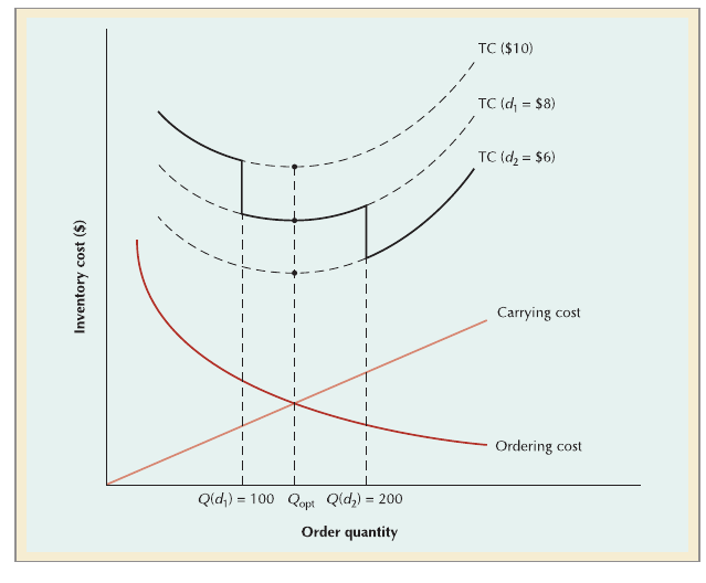
Suppliers often offer a lower unit price if you order in larger quantities. This changes the calculus: total cost must now include the purchase price itself, not just ordering and carrying cost — because a big-enough discount on price might outweigh the extra carrying cost of holding a bigger-than-EOQ order. The quantity discount model tells you exactly when it's worth taking the discount, and when it isn't.
2Formula
where P = per-unit purchase price (which now depends on which price bracket Q falls into).
3When to Use It
Use this model whenever a supplier's price schedule offers a lower per-unit price at higher order quantities, and you must decide whether the basic EOQ or a larger, discounted order size gives the lowest total cost.
4Step-by-Step Method
- Compute the basic EOQ, Qopt = √(2CoD/Cc), ignoring the discount schedule.
- Check which price bracket Qopt falls into, and compute TC (including P·D) at Qopt using that bracket's price.
- For every price bracket below the one containing Qopt (i.e., offering an even lower price at a higher minimum quantity), compute TC at that bracket's minimum qualifying quantity.
- Compare all the computed TC values — the order quantity giving the lowest total cost is the answer, even if it isn't the mathematical Qopt.
5Textbook Example — Example 13.4
Avtek sells TVs with a discount schedule: 1–49 units @ $1,400; 50–89 @ $1,100; 90+ @ $900. Given Co = $2,500, Cc = $190/TV, D = 200 TVs/year:
TC at Q=72.5, P=$1,100: (2,500×200)/72.5 + (190×72.5)/2 + 1,100×200 = $233,784
Since a lower price ($900) is available at 90+ units, also check TC at Q=90, P=$900:
Since $194,105 < $233,784, Avtek should take the maximum discount and order 90 units, even though this is not the mathematical EOQ.
6Important Points
- The purchase price P·D term does not shift the optimal Q within a single price bracket — but it does matter when comparing across brackets.
- Never assume the discount is automatically worth it — you must compare total costs, not just unit prices.
- You only need to check TC at Qopt (in its own bracket) and at the minimum quantity of every cheaper bracket beyond it — not every possible quantity.
7Common Mistakes
- Forgetting to include P·D (purchase cost) in the total cost comparison — this is the whole point of the model.
- Comparing total cost at Qopt using the wrong bracket's price.
- Not checking every cheaper bracket beyond Qopt — only checking one and stopping.