Solved Papers
Every Units 1–6 question from the 2025-26 Final and Re-Examination, cropped from the original paper and worked in full — with the method, the arithmetic in your class's z-table convention, and a check against the official answer key.
Each question shows the original crop from the paper, then a full solution, then a check against the official synoptic answer key. Where the key contains an arithmetic slip, it is flagged rather than copied — there is one such slip, in the Final's Q1 (a).
Questions from Units 7–14 (confidence intervals, hypothesis testing, paired t, F test, ANOVA, chi-square) are not solved here — they are outside the Units 1–6 mid-term portion. They are listed in the Question Bank so you know exactly what was left out.
Your class's table (Standard Normal table.jpg) gives A(z) = the area between 0 and z. The official keys use the cumulative table, Φ(z) = the area to the left of z. They are related by
Every solution below is worked in your class's A(z) convention, then the key's cumulative figures are quoted for comparison. The answers agree. Full table and conversion rules →
Final Q1 (a) — Sampling Distribution of the Mean 2 marks · Unit 5

- Step 1 — Identify what kind of question this is
The phrase "a random sample of 36 different hours will yield a sample mean" is the signal. This is not about one hour — it is about the average of 36. So the sampling distribution of the mean applies, and the denominator must be the standard error, not σ.
μ = 520 σ = 25 n = 36 ⟹ μx̄ = 520 - Step 2 — Standard error σx̄ = σ/√n = 25/√36 = 25/6 = 4.17
- Step 3 — Standardise both ends
z₁ = (515 − 520)/4.17 = −5/4.17 = −1.20
z₂ = (525 − 520)/4.17 = +5/4.17 = +1.20
The interval is symmetric about the mean — which it always is in this slot, because the question is always written as μ ± the same amount.
- Step 4 — Read the table
The region spans the mean, so add the two half-areas:
P(−1.20 < Z < 1.20) = A(1.20) + A(1.20) = 2 × 0.3849 = 0.7698 - Answer
There is a 76.98% chance that a sample of 36 hours averages between 515 and 525 passengers.
The key writes Key p. 1:
The 0.7698 in that line should be 0.8849 — it is Φ(1.20), the cumulative area to the left of 1.20. The correct working is Φ(1.20) − Φ(−1.20) = 0.8849 − 0.1151 = 0.7698. Someone typed the final answer into the first slot and then subtracted from it anyway.
The right answer is 0.7698, and the two cross-checks confirm it: the Re-Exam's identical question gives 0.9250 by the same route with no slip, and 2 × A(1.20) = 0.7698 in your class's table. Write 0.7698.
Re-Exam Q1 (a) — Sampling Distribution of the Mean 2 marks · Unit 5

- Step 1 — Identify what kind of question this is
The phrase "a random sample of 36 different hours will yield a sample mean" is the signal. This is not about one hour — it is about the average of 36. So the sampling distribution of the mean applies, and the denominator must be the standard error, not σ.
μ = 520 σ = 25 n = 36 ⟹ μx̄ = 520 - Step 2 — Standard error σx̄ = σ/√n = 25/√36 = 25/6 = 4.17
- Step 3 — Standardise both ends
z₁ = (515 − 520)/4.17 = −5/4.17 = −1.20
z₂ = (525 − 520)/4.17 = +5/4.17 = +1.20
The interval is symmetric about the mean — which it always is in this slot, because the question is always written as μ ± the same amount.
- Step 4 — Read the table
The region spans the mean, so add the two half-areas:
P(−1.20 < Z < 1.20) = A(1.20) + A(1.20) = 2 × 0.3849 = 0.7698 - Answer
There is a 76.98% chance that a sample of 36 hours averages between 515 and 525 passengers.
The key writes Key p. 1:
The 0.7698 in that line should be 0.8849 — it is Φ(1.20), the cumulative area to the left of 1.20. The correct working is Φ(1.20) − Φ(−1.20) = 0.8849 − 0.1151 = 0.7698. Someone typed the final answer into the first slot and then subtracted from it anyway.
The right answer is 0.7698, and the two cross-checks confirm it: the Re-Exam's identical question gives 0.9250 by the same route with no slip, and 2 × A(1.20) = 0.7698 in your class's table. Write 0.7698.
Re-Exam Q1 (a) — Sampling Distribution of the Mean 2 marks · Unit 5
- Step 1 — Identify what kind of question this is
The phrase "a random sample of 36 different hours will yield a sample mean" is the signal. This is not about one hour — it is about the average of 36. So the sampling distribution of the mean applies, and the denominator must be the standard error, not σ.
μ = 520 σ = 25 n = 36 ⟹ μx̄ = 520 - Step 2 — Standard error σx̄ = σ/√n = 25/√36 = 25/6 = 4.17
- Step 3 — Standardise both ends
z₁ = (515 − 520)/4.17 = −5/4.17 = −1.20
z₂ = (525 − 520)/4.17 = +5/4.17 = +1.20
The interval is symmetric about the mean — which it always is in this slot, because the question is always written as μ ± the same amount.
- Step 4 — Read the table
The region spans the mean, so add the two half-areas:
P(−1.20 < Z < 1.20) = A(1.20) + A(1.20) = 2 × 0.3849 = 0.7698 - Answer
There is a 76.98% chance that a sample of 36 hours averages between 515 and 525 passengers.
The key writes Key p. 1:
The 0.7698 in that line should be 0.8849 — it is Φ(1.20), the cumulative area to the left of 1.20. The correct working is Φ(1.20) − Φ(−1.20) = 0.8849 − 0.1151 = 0.7698. Someone typed the final answer into the first slot and then subtracted from it anyway.
The right answer is 0.7698, and the two cross-checks confirm it: the Re-Exam's identical question gives 0.9250 by the same route with no slip, and 2 × A(1.20) = 0.7698 in your class's table. Write 0.7698.
Re-Exam Q1 (a) — Sampling Distribution of the Mean 2 marks · Unit 5
- Step 1 — Set up μ = 240 σ = 18 n = 64 ⟹ μx̄ = 240
- Step 2 — Standard error σx̄ = 18/√64 = 18/8 = 2.25
- Step 3 — Standardise z₁ = (236 − 240)/2.25 = −4/2.25 = −1.78 z₂ = (244 − 240)/2.25 = +1.78
- Step 4 — Read the table and add P(−1.78 < Z < 1.78) = 2 × A(1.78) = 2 × 0.4625 = 0.9250
- Answer
92.5% chance the sample of 64 days averages between 236 and 244 calls.
✓ Matches the key exactly: 0.9625 − 0.0375 = 0.9250 Key p. 1. In cumulative terms, Φ(1.78) = 0.9625 and Φ(−1.78) = 0.0375, and 0.9625 = 0.5 + 0.4625 — the same number in the other convention.
Final Q1 (b) — Poisson, P(no arrivals) 4 marks · Unit 4

- Step 1 — Recognise the distribution and say so
"On average, 2 customers arrive… every 10 minutes" is a rate per interval with no fixed number of trials ⟹ Poisson. Write that sentence down; it is worth a mark on a 4-mark question.
Let X = number of customers arriving in a 10-minute interval X ~ Po(λ) - Step 2 — Identify λ for the interval asked about
The rate is given per 10 minutes and the question asks about 10 minutes, so no scaling is needed.
λ = 2 x = 0 - Step 3 — Apply the formula P(X = 0) = e^(−λ)·λˣ / x! = e^(−2) × 2⁰ / 0! = e^(−2) × 1 / 1 = e^(−2)
- Step 4 — Evaluate = 0.1353 or about 13.53%
✓ Matches the key exactly Key p. 1. Note the shortcut it relies on: because λ⁰ = 1 and 0! = 1, P(X = 0) is always just e^(−λ).
Re-Exam Q1 (b) — Poisson, P(at least one) 4 marks · Unit 4

- Step 1 — Set up Let X = number of breakdowns in one day X ~ Po(1.5), so λ = 1.5
- Step 2 — Spot "at least one" and take the complement
Computing P(X = 1) + P(X = 2) + … forever is impossible. The rule of at least one turns it into a single subtraction:
P(X ≥ 1) = 1 − P(X = 0) - Step 3 — Compute P(X = 0) P(X = 0) = e^(−1.5) × 1.5⁰ / 0! = e^(−1.5) = 0.2231
- Step 4 — Subtract P(X ≥ 1) = 1 − 0.2231 = 0.7769 or 77.69%
✓ Matches the key exactly Key p. 1, which lays it out in the same four lines.
Final Q2 (b) — Normal Distribution, Two Parts 5 marks · Unit 4
- Step 1 — Set up, and note there is no n
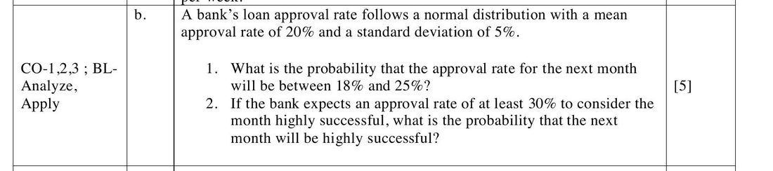
X = approval rate in a month X ~ N(μ = 20, σ = 5)
No sample size is mentioned, so this is about one month, not a mean of several. Divide by σ = 5, not by a standard error. Working in percentage points throughout keeps the arithmetic clean.
- Step 2 — Part 1: P(18 ≤ X ≤ 25)
z₁ = (18 − 20)/5 = −0.40 z₂ = (25 − 20)/5 = +1.00
The interval straddles the mean (one z negative, one positive), so add the two half-areas:
P(−0.40 ≤ Z ≤ 1.00) = A(0.40) + A(1.00) = 0.1554 + 0.3413 = 0.4967About a 49.7% chance the approval rate lands between 18% and 25%.
- Step 3 — Part 2: P(X ≥ 30), "highly successful"
z = (30 − 20)/5 = +2.00
A right tail, so subtract from the half:
P(Z ≥ 2.00) = 0.5 − A(2.00) = 0.5 − 0.4772 = 0.0228Only a 2.28% chance of a highly successful month.
- Step 4 — One business sentence
An approval rate of 30% is two standard deviations above the norm, so "highly successful" months should be expected roughly once every 44 months — the target is set unrealistically high for routine planning.
✓ Matches the key Key p. 2: it computes 0.8413 − 0.3446 = 0.4967 and 1 − 0.9772 = 0.0228 in the cumulative convention. Same answers, other table.
Re-Exam Q2 (b) — Normal Distribution, Two Parts 5 marks · Unit 4
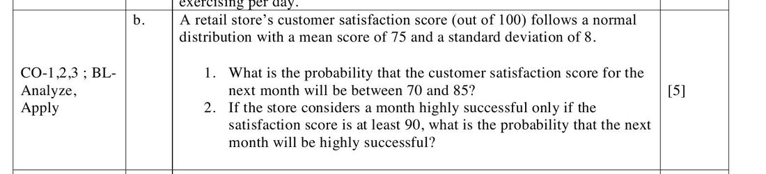
- Step 1 — Set up X = monthly satisfaction score X ~ N(μ = 75, σ = 8)
- Step 2 — Part 1: P(70 ≤ X ≤ 85)
z₁ = (70 − 75)/8 = −5/8 = −0.625 z₂ = (85 − 75)/8 = 10/8 = +1.25
Straddles the mean, so add. Standard tables step in hundredths, so round −0.625 to −0.63:
P(−0.63 ≤ Z ≤ 1.25) = A(0.63) + A(1.25) = 0.2357 + 0.3944 = 0.6301The key interpolates at the exact −0.625 and gets 0.6284 Key p. 2. Both are correct to two decimals; say which z you rounded to.
- Step 3 — Part 2: P(X ≥ 90), "highly successful"
z = (90 − 75)/8 = 15/8 = +1.875 → round to 1.88
P(Z ≥ 1.88) = 0.5 − A(1.88) = 0.5 − 0.4699 = 0.0301
The key gives 1 − 0.9694 = 0.0306 using the exact 1.875 Key p. 2.
- Step 4 — Business sentence
Only about 3% of months will clear the score of 90. Around 63% land in the ordinary 70–85 band, so the store's normal operating range is the one to manage against.
The Re-Exam produces z = −0.625 and z = 1.875, which fall exactly halfway between table rows. State your rounding — "taking z ≈ 1.88" — and the answer will be accepted. Do not silently invent a third decimal that is not in the table you were given.
Final Q3 (a) — Interpreting Descriptive Statistics 5 marks · Units 1–2
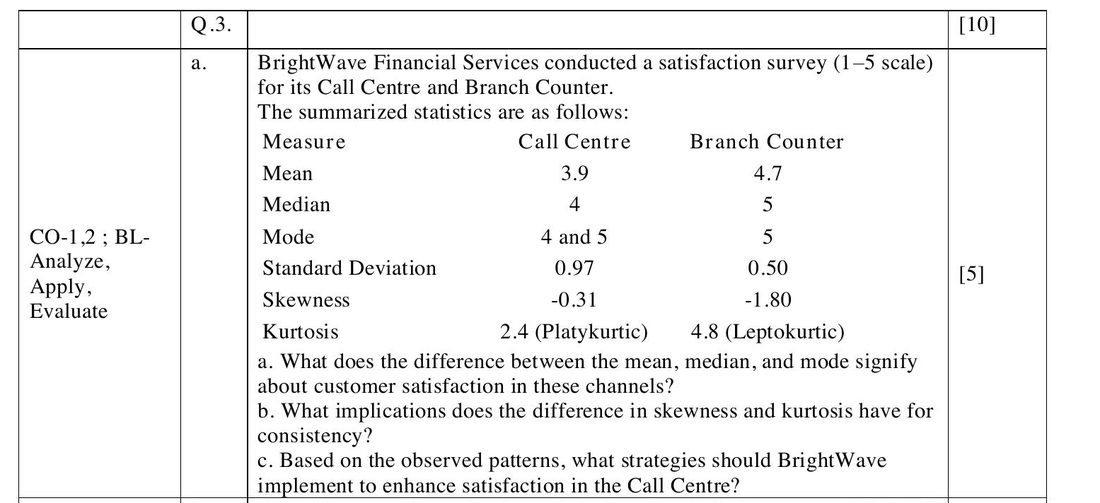
(a) What does the difference between mean, median and mode signify?
| Channel | Ordering | Shape | Reading |
|---|---|---|---|
| Call Centre | Mean 3.9 < Median 4 ≈ Mode 4 and 5 | Mild negative skew (−0.31) | Most customers are moderately satisfied (scores 4–5), but a minority of low ratings pulls the mean down below the median. |
| Branch Counter | Mean 4.7 < Median 5 = Mode 5 | Strong negative skew (−1.80) | The majority are highly satisfied, with scores concentrated near 5. Only a very small tail of dissatisfied customers. |
The general rule doing the work here: Mean < Median ≤ Mode ⟹ negatively skewed ⟹ a left tail of low scores. The bigger the gap between mean and median, the heavier that tail. Branch Counter's gap of 0.3 with skewness −1.80 is far more extreme than Call Centre's 0.1 with −0.31.
Note the Call Centre is bimodal — mode "4 and 5". Say so: it means customer opinion is split between two clusters rather than settling on one typical experience.
(b) What do skewness and kurtosis imply for consistency?
| Measure | Call Centre | Branch Counter | Meaning |
|---|---|---|---|
| Standard deviation | 0.97 | 0.50 | Branch Counter's SD is roughly half — its ratings vary far less. |
| Skewness | −0.31 | −1.80 | Branch's distribution is far more concentrated at the top of the scale. |
| Kurtosis | 2.4 — platykurtic (K < 3) | 4.8 — leptokurtic (K > 3) | Flat and spread out vs tall and narrow. |
High SD + LOW kurtosis (platykurtic): INCONSISTENT, variable service
So: the Branch Counter delivers a uniformly excellent experience (SD 0.50, leptokurtic 4.8 — ratings tightly clustered around 5), while the Call Centre is inconsistent (SD 0.97, platykurtic 2.4 — a flatter curve with ratings spread across the scale). Two customers of the Call Centre can have completely different experiences; two customers of the Branch Counter almost certainly will not.
(c) What strategies should BrightWave implement for the Call Centre?
Each strategy must be tied to the statistic that justifies it — that link is what earns the marks:
- Reduce variability (attacks the SD of 0.97): standardise call scripts and resolution procedures so every agent handles a call the same way.
- Address the left tail (attacks the −0.31 skew): identify and fix the causes of the low ratings specifically — long wait times, unresolved first contacts.
- Raise kurtosis toward the leptokurtic shape (targets the 2.4): continuous agent training, feedback loops after poor scores, and rewards for consistent performers rather than for peak performance.
- Monitor the metrics themselves: track mean, SD, skewness and kurtosis monthly, with an explicit goal of raising the mean, cutting the SD, moving skewness toward 0 and lifting kurtosis.
✓ Every point above appears in the official key Key p. 3, which is structured under exactly these three headings.
Re-Exam Q3 (a) — Interpreting Descriptive Statistics 5 marks · Units 1–2
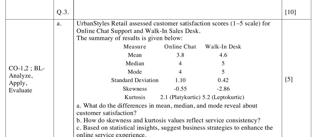
Structurally identical to the Final's version — the same six statistics for two channels, the same three sub-parts. Only the story and the numbers change.
(a) Mean, median and mode
| Channel | Mean | Median | Mode | Reading |
|---|---|---|---|---|
| Online Chat | 3.8 | 4 | 4 | Mean < Median = Mode ⟹ moderate negative skew (−0.55). Many customers are satisfied, but a noticeable number report poor experiences and pull the mean down. |
| Walk-In Desk | 4.6 | 5 | 5 | Mean < Median = Mode ⟹ strong negative skew (−2.86). Almost all customers are extremely satisfied. |
(b) Skewness and kurtosis — service consistency
- Online Chat: high SD 1.10, kurtosis 2.1 → platykurtic, a flat wide curve. High variability means inconsistent service delivery.
- Walk-In Desk: low SD 0.42, kurtosis 5.2 → leptokurtic, a tall narrow peak. Strong consistency and reliability.
Note how much more extreme this pair is than the Final's: skewness −2.86 and kurtosis 5.2 describe a distribution almost entirely piled on the value 5.
(c) Strategies to improve the online service experience
- Reduce dispersion and the left tail: identify outlier cases — long waits, poor chatbot responses — and provide agent-escalation training so a stuck chat reaches a human quickly.
- Enhance consistency: standardised response templates; improve the chatbot-to-human handoff; measure and reward consistent service quality rather than one-off excellence.
- Raise the mean and the kurtosis: set explicit service-quality KPIs (response time ≤ 2 minutes, first-contact resolution ≥ 90%) and track skewness and kurtosis monthly to confirm ratings are clustering nearer 4–5.
✓ Every point appears in the key Key p. 2.
Final Q3 (b) — Sample Size for a Mean 5 marks · Unit 6

- Step 1 — Which formula? Mean or proportion?
The quantity being estimated is a mean cholesterol level in mg/dL — a measured average, not a percentage of people. And a population σ is supplied. So this is the mean formula.
- Step 2 — Extract the three inputs
σ = 32 mg/dL E = 5 mg/dL confidence = 99% ⟹ z0.005 = 2.576
99% leaves 1% in the two tails combined, so 0.5% in each — hence the subscript 0.005. Do not reach for 1.96 out of habit.
- Step 3 — Substitute into n = (z·σ / E)² n = (2.576 × 32 / 5)² = (82.432 / 5)² = (16.4864)²
- Step 4 — Evaluate and round UP
= 271.8 ⟹ n = 272 adults
Round up, always. 271 people would give a margin of error slightly wider than the 5 mg/dL promised.
- Step 5 — State the answer in words
The agency must sample at least 272 adults to be 99% confident the sample mean is within 5 mg/dL of the true mean cholesterol level.
✓ Matches the key, which writes n ≈ 271.9 → n = 272 Key p. 3. The 0.1 difference is rounding inside 2.576 × 32; both round to 272.
Re-Exam Q3 (b) — Sample Size for a Proportion, No Prior Estimate 5 marks · Unit 6

- Step 1 — Which formula?
The quantity being estimated is the proportion of consumers who prefer online shopping — a percentage of people. So this is the proportion formula, n = z²pq / E².
- Step 2 — Handle the missing p, and justify it in writing
The formula needs p, but "no prior estimate of the population proportion is available". The convention:
Take p = 0.5 (hence q = 0.5), because p·q is maximised at p = 0.5Write the reason out: "With no prior estimate, p = 0.5 is used because it gives maximum variability (pq = 0.25) and therefore the largest — that is, the safest — required sample size." That sentence is a mark on its own.
- Step 3 — Inputs
z = 1.96 (95%) E = 0.04 p = q = 0.5
±0.04 means E = 0.04, not 4. Keep proportions as decimals throughout.
- Step 4 — Substitute n = z²·p·q / E² = (1.96)² × 0.5 × 0.5 / (0.04)² = 3.8416 × 0.25 / 0.0016 = 0.9604 / 0.0016
- Step 5 — Evaluate and round UP = 600.25 ⟹ n = 601 consumers
- Step 6 — Interpret
To estimate the proportion preferring online shopping with 95% confidence and a margin of error of ±0.04, the firm should sample at least 601 people.
✓ Matches the key line for line, including the round-up from 600.25 to 601 Key p. 3.
Final Q4 (a) — Finite Population Correction 5 marks · Unit 5 half in scope
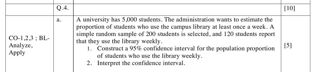
This question builds a confidence interval, which is Unit 7 and outside the mid-term portion. But the standard error it needs uses the finite population correction from Unit 5, and the whole question is a natural extension of the sampling distribution of a proportion. It is worked in full here — treat the CI half as a preview.
- Step 1 — Extract and compute the sample proportion N = 5,000 n = 200 x = 120 ⟹ p̂ = 120/200 = 0.60, q̂ = 0.40
- Step 2 — Standard error with the FPC
SE = √[ p̂(1−p̂)/n × (N − n)/(N − 1) ]
= √[ (0.6 × 0.4)/200 × (5000 − 200)/(5000 − 1) ]
= √[ 0.0012 × 4800/4999 ] = √[0.0012 × 0.9602] = √0.001152 = 0.03395
The multiplier √0.9602 = 0.9799 shaved about 2% off the standard error. Strictly, n/N = 200/5000 = 0.04 is below the 0.05 threshold, so the correction was optional — but the key applies it because the question hands you N, and so should you.
- Step 3 — Margin of error E = zα/2 × SE = 1.96 × 0.03395 = 0.0666
- Step 4 — Confidence interval CI = p̂ ± E = 0.60 ± 0.0666 = (0.533, 0.667)
- Step 5 — Interpret (part 2 of the question)
"We are 95% confident that between 53.3% and 66.7% of all 5,000 students use the campus library at least once a week." Say 95% confident, never "there is a 95% probability that the true proportion lies here" — the true proportion is a fixed number, it is the interval that varies from sample to sample.
✓ Matches the key exactly Key p. 4.
Re-Exam Q4 (a) — Finite Population Correction 5 marks · Unit 5 half in scope
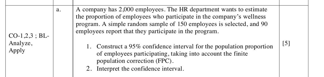
Note that this version names the FPC in the question itself — "taking into account the finite population correction (FPC)" — so there is no judgement call to make.
- Step 1 — Extract
N = 2,000 n = 150 x = 90 ⟹ p̂ = 90/150 = 0.60, q̂ = 0.40
Check the sampling fraction: n/N = 150/2000 = 0.075 > 0.05, so the FPC genuinely matters here.
- Step 2 — Standard error with the FPC SE = √[ (0.6 × 0.4)/150 × (2000 − 150)/(2000 − 1) ] = √[ 0.0016 × 1850/1999 ] = √[0.0016 × 0.9255] = √0.0014808 = 0.03848
- Step 3 — Margin of error and interval E = 1.96 × 0.03848 = 0.0754 CI = 0.60 ± 0.0754 = (0.525, 0.675)
- Step 4 — Interpret
"We are 95% confident that between 52.5% and 67.5% of the company's 2,000 employees participate in the wellness programme."
✓ Matches the key exactly Key p. 3.
Final Q5 (a) — Bayes' Theorem on a Credit Model 5 marks · Unit 3
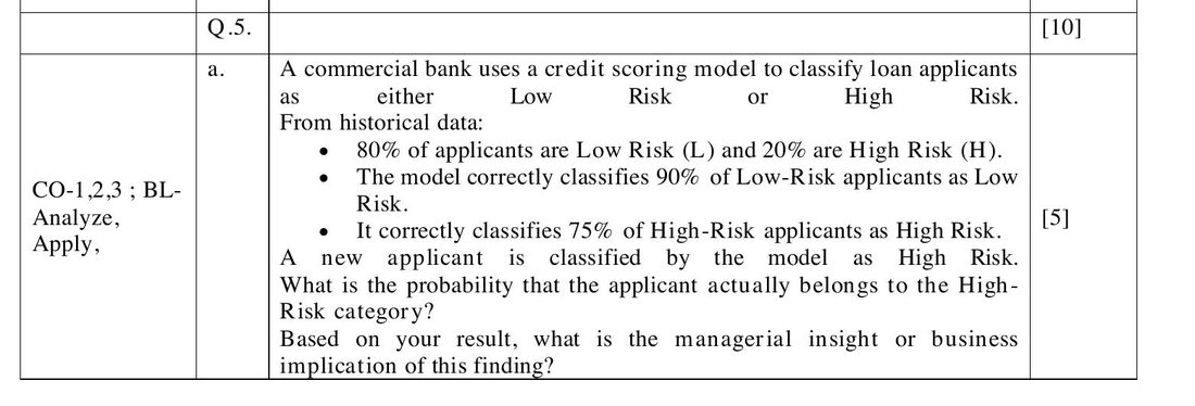
- Step 1 — Define the events in words
L = applicant is genuinely Low Risk H = applicant is genuinely High Risk
T = the model classifies the applicant as High Risk
Keeping "what the applicant is" separate from "what the model says" is the whole battle in this question.
- Step 2 — Write down the given probabilities, converting where needed
Words in the question Symbol Value 80% of applicants are Low Risk P(L) 0.80 20% are High Risk P(H) 0.20 Correctly classifies 75% of High-Risk as High Risk P(T | H) 0.75 Correctly classifies 90% of Low-Risk as Low Risk — so it wrongly flags the other 10% P(T | L) 1 − 0.90 = 0.10 That last row is the trap. The question hands you the true-negative rate; the formula needs the false-positive rate. Subtract.
- Step 3 — Law of total probability: how often does the model say "High Risk" at all?
P(T) = P(L)·P(T|L) + P(H)·P(T|H)
= (0.80)(0.10) + (0.20)(0.75) = 0.08 + 0.15 = 0.23
23% of all applicants get flagged. Of that 23 percentage points, 15 are genuine and 8 are false alarms — the answer is already visible.
- Step 4 — Bayes' theorem P(H | T) = P(H)·P(T|H) / P(T) = 0.15 / 0.23 = 0.652
- Step 5 — Managerial insight — do not skip this
The prior was 20%; after the model flags someone it rises to 65.2%. The model is genuinely informative — it more than triples the odds. But 34.8%, roughly 1 in 3, of flagged applicants are false alarms.
So: "Even though the model classifies an applicant as high risk, about 1 in 3 such classifications are false alarms. The bank should not reject automatically — borderline flagged cases should be reviewed manually before a decision, or the bank will turn away creditworthy customers."
✓ Matches the key, whose insight paragraph is almost word for word the sentence above Key p. 4.
Re-Exam Q5 (a) — Bayes' Theorem on a Churn Model 5 marks · Unit 3
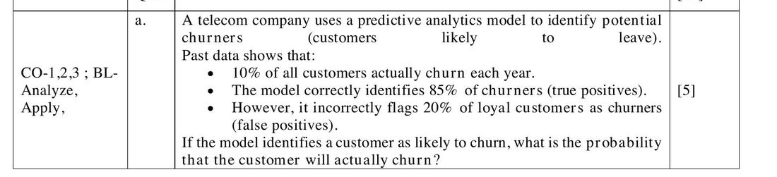
- Step 1 — Define C = customer genuinely churns L = customer is genuinely loyal P = the model predicts churn (flags the customer)
- Step 2 — Given probabilities — and note the difference from the Final
Words in the question Symbol Value 10% of all customers actually churn P(C) 0.10 Therefore P(L) 0.90 Correctly identifies 85% of churners (true positives) P(P | C) 0.85 Incorrectly flags 20% of loyal customers (false positives) P(P | L) 0.20 — no subtraction Here the question gives the false-positive rate directly. The Final gave the true-negative rate. Read which one you have been handed before you write anything.
- Step 3 — Total probability of a flag
P(P) = P(C)·P(P|C) + P(L)·P(P|L)
= (0.10)(0.85) + (0.90)(0.20) = 0.085 + 0.18 = 0.265
Look at the split: only 0.085 of that 0.265 is genuine. The false positives, drawn from the much larger loyal group, outnumber the true positives two to one.
- Step 4 — Bayes P(C | P) = 0.085 / 0.265 = 0.321
- Step 5 — Managerial insight
The prior was 10%; a flag raises it to 32.1% — a threefold increase, so the model is useful. But only about one-third of flagged customers actually churn.
"Targeted retention offers should focus on this smaller genuine segment to optimise marketing spend, rather than giving discounts to all flagged users — two-thirds of whom would have stayed anyway."
✓ Matches the key Key p. 4.
Final Q5 (b) — Standard Error and a One-Tail Probability 5 marks · Units 5–6

- Step 1 — Tabulate what you have (the key does this, and it reads well)
Parameter Symbol Value Population mean μ 2.5 days Population standard deviation σ 0.5 days Sample size n 64 Mean of the sampling distribution μx̄ = μ 2.5 days - Step 2 — Part 1: the standard error (asked for explicitly)
σx̄ = σ/√n = 0.5/√64 = 0.5/8 = 0.0625 days
Give it as its own labelled answer — the question numbers it as sub-part 1, so it carries its own marks.
- Step 3 — Part 2: P(x̄ < 2.4) z = (x̄ − μx̄)/σx̄ = (2.4 − 2.5)/0.0625 = −0.1/0.0625 = −1.60
- Step 4 — Read the table — a left tail P(Z < −1.60) = 0.5 − A(1.60) = 0.5 − 0.4452 = 0.0548
- Step 5 — Answer and one business line
There is a 5.48% chance that 64 randomly chosen deliveries average under 2.4 days. So if the regional manager does observe an average of 2.4 days, that is unusual enough to suggest the branch is genuinely faster than the company's 2.5-day claim, rather than just lucky.
✓ Matches the key exactly, including the 0.0625 and the 0.0548 Key p. 5.
Re-Exam Q5 (b) — Standard Error and an Interval Probability 5 marks · Units 5–6
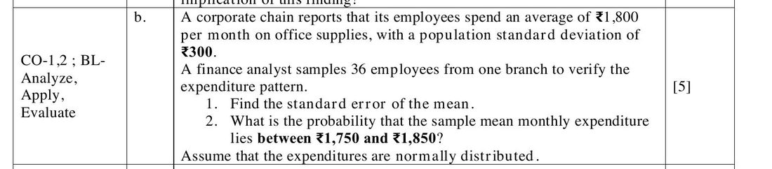
- Step 1 — Set up μ = ₹1,800 σ = ₹300 n = 36 ⟹ μx̄ = ₹1,800
- Step 2 — Part 1: standard error σx̄ = 300/√36 = 300/6 = ₹50
- Step 3 — Part 2: standardise both ends
z₁ = (1750 − 1800)/50 = −50/50 = −1.00
z₂ = (1850 − 1800)/50 = +50/50 = +1.00
A symmetric interval about the mean again — exactly the Q1 (a) shape, now worth 5 marks instead of 2.
- Step 4 — Read the table and add P(−1.00 < Z < 1.00) = 2 × A(1.00) = 2 × 0.3413 = 0.6826
- Step 5 — Answer and interpretation
There is a 68.26% chance the 36-employee sample averages between ₹1,750 and ₹1,850.
Worth noticing: ±₹50 is exactly ±1 standard error, so this is the empirical rule's 68% appearing on cue. If you see z = ±1, you can quote 68.26% without touching the table — and the same trick gives 95.44% at z = ±2 and 99.74% at z = ±3.
✓ Matches the key exactly: 0.8413 − 0.1587 = 0.6826 Key p. 4.
The scoreboard — what Units 1–6 are worth
| Slot | Topic | Unit | Marks | In scope? |
|---|---|---|---|---|
| Q1 (a) | Sampling distribution of the mean | 5 | 2 | Yes |
| Q1 (b) | Poisson | 4 | 4 | Yes |
| Q1 (c) | Type I and Type II errors | 9 | 4 | No — hypothesis testing |
| Q2 (a) | Confidence interval for a mean | 7–8 | 5 | No — estimation |
| Q2 (b) | Normal distribution | 4 | 5 | Yes |
| Q3 (a) | Interpreting descriptive statistics | 1–2 | 5 | Yes |
| Q3 (b) | Sample size determination | 6 | 5 | Yes |
| Q4 (a) | CI for a proportion, with the FPC | 5 + 7 | 5 | Half — the FPC is Unit 5 |
| Q4 (b) | Hypothesis test of a proportion | 10 | 5 | No |
| Q5 (a) | Bayes' theorem | 3 | 5 | Yes |
| Q5 (b) | Standard error and P(x̄) | 5–6 | 5 | Yes |
| Q6 (a) | Paired t-test output | 11 | 5 | No |
| Q6 (b) | F test for two variances | 12 | 5 | No |
| Q7 (a) | One-way ANOVA output | 13 | 5 | No |
| Q7 (b) | Chi-square test of independence | 14 | 5 | No |
| Units 1–6 total | 31 | + 5 half | ||
Marks sum to more than 50 because Q1 is compulsory and you then choose any 4 of Q2–Q7. The point stands: in both papers there was enough Units 1–6 material to build most of a complete answer script.