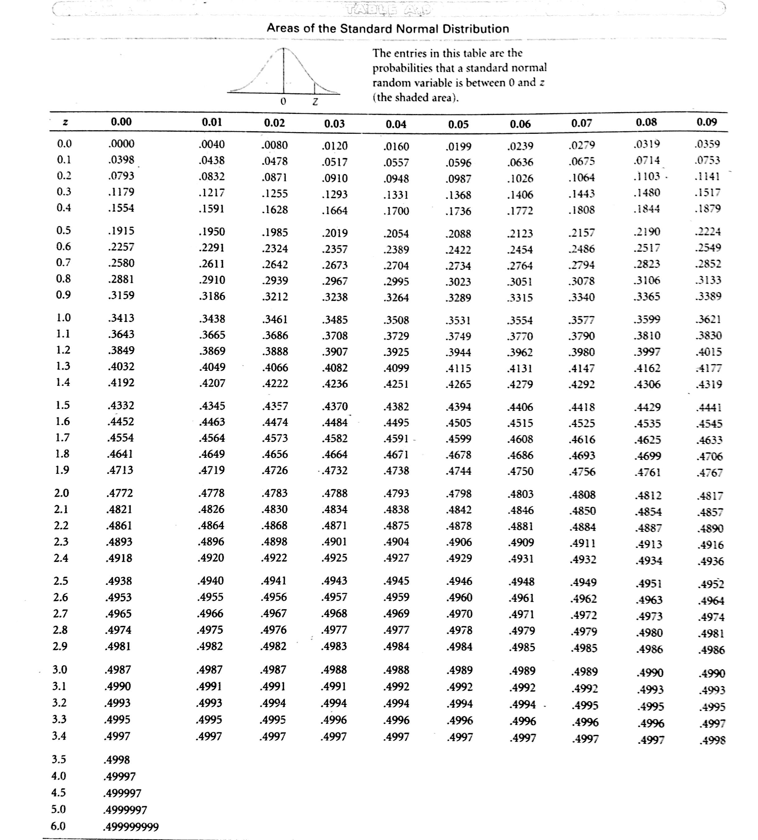
Every formula in Units 1–6 on one page, in the order you will need them — plus the standard normal table your class actually uses, and the rules for reading it.
◆ If you only memorise six things
1. Standard error
\[ \sigma_{\bar{x}} = \frac{\sigma}{\sqrt{n}} \qquad \text{(7 marks in both papers)} \]
2. Standardising sample mean
\[ z = \frac{\bar{x} - \mu}{\sigma_{\bar{x}}} \]
3. Poisson distribution
\[ P(X = x) = \frac{e^{-\lambda}\lambda^x}{x!} \qquad \text{and } P(X=0) = e^{-\lambda} \]
4. Bayes' theorem
\[ P(S_i \mid A) = \frac{P(S_i)P(A \mid S_i)}{\sum P(S_i)P(A \mid S_i)} \]
5. Sample size (mean)
\[ n = \left(\frac{z \cdot \sigma}{E}\right)^2 \]
6. Sample size (proportion)
\[ n = \frac{z^2 p q}{E^2} \qquad \text{(with } p = 0.5 \text{ if unknown)} \]
Those six cover 26 of the 31 in-scope marks. The remaining 5 are Q3 (a), which needs no formula at all — only the reading rules in §2 below.
Units 1–2 — Descriptive Statistics
Central tendency
Population & sample mean
\[ \mu = \frac{\sum x}{N} \qquad \bar{x} = \frac{\sum x}{n} \]
Grouped mean (frequency table)
\[ \bar{x} \text{ or } \mu = \frac{\sum f \cdot x}{\sum f} \qquad \text{where } x = \text{class midpoint} = \frac{\text{lower} + \text{upper}}{2} \]
Median & Mode
\[ \text{Median} = \text{middle value once ordered} \qquad \text{Mode} = \text{most frequent value} \]
Class-notes rule: an inclusive series (1–3, 4–6, …) need not be converted to exclusive for the MEAN, but conversion is required for the MEDIAN and MODE Class notes p. 3.
Dispersion
Range
\[ \text{Range} = \text{Highest} - \text{Lowest} \]
Population variance & SD
\[ \sigma^2 = \frac{\sum (x - \mu)^2}{N} \qquad \sigma = \sqrt{\sigma^2} \]
Sample variance & SD
\[ s^2 = \frac{\sum (x - \bar{x})^2}{n - 1} \qquad s = \sqrt{s^2} \]
Grouped variance
\[ \sigma^2 = \frac{\sum f(x - \mu)^2}{\sum f} \qquad s^2 = \frac{\sum f(x - \bar{x})^2}{\sum f - 1} \]
Coefficient of Variation
\[ \text{CV} = \left(\frac{\sigma}{\bar{x}}\right) \times 100\% \]
÷ N for a POPULATION. ÷ (n − 1) for a SAMPLE. Nothing to do with dataset size.
Skewness, kurtosis and the shape rules
Karl Pearson 1st Skewness
\[ Sk = \frac{\text{Mean} - \text{Mode}}{SD} \]
Karl Pearson 2nd Skewness
\[ Sk = \frac{3(\text{Mean} - \text{Median})}{SD} \]
Bowley Quartile Skewness
\[ Sk = \frac{Q_3 + Q_1 - 2 Q_2}{Q_3 - Q_1} \]
Reading Skewness
\[ \text{Mean} < \text{Median} \le \text{Mode} \implies \text{Negative (left tail)} \qquad \text{Mean} > \text{Median} \ge \text{Mode} \implies \text{Positive (right tail)} \]
Kurtosis Benchmark
\[ K > 3 \implies \text{Leptokurtic (consistent)} \qquad K = 3 \implies \text{Mesokurtic (normal)} \qquad K < 3 \implies \text{Platykurtic (flat)} \]
Excel's KURT() reports excess kurtosis and benchmarks against 0, not 3. Both papers use the K-vs-3 convention.
Chebyshev and the empirical rule
Chebyshev (Any Dist)
\[ \text{At least } \left(1 - \frac{1}{k^2}\right) \text{ inside } \mu \pm k\sigma \qquad (k=2 \implies 75\%, \; k=3 \implies 89\%) \]
Empirical Rule (Normal)
\[ \mu \pm 1\sigma \approx 68.26\% \qquad \mu \pm 2\sigma \approx 95.44\% \qquad \mu \pm 3\sigma \approx 99.74\% \]
To convert a percentage into a COUNT: multiply by the total number of observations.
Choosing the chart
Qualitative data
\[ \text{Tabular: Frequency / Relative / Percent / Crosstab} \qquad \text{Graphs: Bar Graph (separated) / Pie Chart} \]
Quantitative data
\[ \text{Tabular: Cumulative / Relative} \qquad \text{Graphs: Histogram (touching) / Ogive / Stem-and-Leaf / Scatter} \]
Pie slice angle
\[ \text{Angle} = \text{Relative Frequency} \times 360^\circ \]
Unit 3 — Probability
The rules
Complement
\[ P(A^c) = 1 - P(A) \]
Addition ("or")
\[ P(A \cup B) = P(A) + P(B) - P(A \cap B) \qquad \text{(Mutually exclusive: } P(A \cup B) = P(A) + P(B)\text{)} \]
Multiplication ("and")
\[ P(A \cap B) = P(B) \cdot P(A \mid B) \qquad \text{(Independent: } P(A \cap B) = P(A) \cdot P(B)\text{)} \]
Conditional Probability
\[ P(A \mid B) = \frac{P(A \cap B)}{P(B)} \]
Independence Test
\[ A \text{ and } B \text{ independent } \iff P(A \cap B) = P(A) \cdot P(B) \]
Rule of At Least One
\[ P(\text{at least one}) = 1 - P(\text{none}) = 1 - (1-p_1)(1-p_2)\dots(1-p_n) = 1 - (1-p)^n \]
Expected Successes
\[ E = \sum p_i \qquad \text{or} \qquad E = n \cdot p \]
Counting
Multi-step Experiments
\[ \text{Total outcomes} = n_1 \cdot n_2 \dots n_k \]
Combinations (Order doesn't matter)
\[ C(N,n) = \binom{N}{n} = \frac{N!}{n!(N-n)!} \]
Permutations (Order matters)
\[ P(N,n) = \frac{N!}{(N-n)!} \]
Total probability and Bayes
Law of Total Probability
\[ P(A) = P(S_1)P(A \mid S_1) + P(S_2)P(A \mid S_2) + \dots + P(S_k)P(A \mid S_k) \]
Bayes' Theorem
\[ P(S_i \mid A) = \frac{P(S_i) \cdot P(A \mid S_i)}{\sum P(S_i) \cdot P(A \mid S_i)} = \frac{\text{One branch}}{P(A)} \]
FIVE-LINE METHOD FOR BAYES:
1. Define events in words · 2. List priors and conditionals · 3. Total probability P(A) · 4. Bayes: one branch ÷ P(A) · 5. Managerial insight (carries marks)
Unit 4 — Probability Distributions
Expected value and variance
Expected Value (Discrete)
\[ E(X) = \mu = \sum x \cdot P(x) \]
Variance of Random Variable
\[ \text{Var}(X) = \sigma^2 = \sum (x - \mu)^2 P(x) = \sum x^2 P(x) - \mu^2 \]
Binomial
Binomial Probability
\[ P(X = r) = \binom{n}{r} p^r (1-p)^{n-r} = \frac{n!}{r!(n-r)!} p^r q^{n-r} \]
Mean & SD
\[ \mu = np \qquad \sigma^2 = npq \qquad \sigma = \sqrt{npq} \]
Excel: =BINOM.DIST(r, n, p, FALSE) (exact r) · =BINOM.DIST(r, n, p, TRUE) (r or fewer)
Poisson
Poisson Probability
\[ P(X = x) = \frac{e^{-\lambda} \lambda^x}{x!} \qquad \mu = \lambda, \; \sigma^2 = \lambda, \; \sigma = \sqrt{\lambda} \]
Poisson Workhorses
\[ P(X = 0) = e^{-\lambda} \qquad P(X \ge 1) = 1 - e^{-\lambda} \]
Rescaling & Binomial Approx
\[ \lambda_{\text{new}} = \lambda_{\text{given}} \times \frac{\text{new interval}}{\text{given interval}} \qquad \lambda = np \quad (n \ge 20, \; p \le 0.05) \]
Excel: =POISSON.DIST(x, λ, FALSE) (exact x) · =POISSON.DIST(x, λ, TRUE) (x or fewer)
Normal
Standardising (Z)
\[ z = \frac{x - \mu}{\sigma} \qquad \text{for ONE observation} \]
Continuity Correction
\[ z = \frac{(r \pm 0.5) - np}{\sqrt{npq}} \qquad \text{(valid when } np \ge 5 \text{ and } nq \ge 5\text{)} \]
◆ Which distribution? — the 10-second decision
Fixed n, 2 outcomes, p constant
\[ \text{BINOMIAL} \qquad P(X=r) = \binom{n}{r} p^r q^{n-r} \]
Average RATE per interval
\[ \text{POISSON} \qquad P(X=x) = \frac{e^{-\lambda}\lambda^x}{x!} \]
Continuous measurement
\[ \text{NORMAL} \qquad z = \frac{x - \mu}{\sigma} \]
Sample mean x̄
\[ \text{NORMAL WITH STANDARD ERROR} \qquad z = \frac{\bar{x} - \mu}{\sigma / \sqrt{n}} \]
Units 5–6 — Sampling Theory
Notation — get this right and the formulas follow
| Quantity | Population
(parameter) | Sample
(statistic) | Sampling distribution |
|---|
| Mean | μ | x̄ | μx̄ = μ · σx̄ |
| Standard deviation | σ | s | σx̄ = the standard error |
| Proportion | p | p̂ | μp̂ = p · σp̂ |
| Size | N | n | — |
Standard error and standardising
Standard error of mean
\[ \sigma_{\bar{x}} = \frac{\sigma}{\sqrt{n}} \qquad z = \frac{\bar{x} - \mu}{\sigma_{\bar{x}}} \qquad (\mu_{\bar{x}} = \mu) \]
Standard error of proportion
\[ \sigma_{\hat{p}} = \sqrt{\frac{p q}{n}} \qquad z = \frac{\hat{p} - p}{\sigma_{\hat{p}}} \qquad (\mu_{\hat{p}} = p, \; np \ge 5, \; nq \ge 5) \]
Finite Population Multiplier
\[ \text{FPM} = \sqrt{\frac{N - n}{N - 1}} \qquad \sigma_{\bar{x}} = \frac{\sigma}{\sqrt{n}} \times \sqrt{\frac{N - n}{N - 1}} \]
Skip FPM when sampling fraction n/N < 0.05. If N is given in the question, apply it and state why.
Central Limit Theorem
CLT Statement
\[ \text{For any population shape, as } n \ge 30, \; \bar{x} \sim N\left(\mu, \; \frac{\sigma}{\sqrt{n}}\right) \]
Why it matters: It lets you use sample statistics to infer population parameters without knowing the population's underlying distribution shape.
Margin of error, precision and sample size
Margin of error (E)
\[ E = z \cdot \frac{\sigma}{\sqrt{n}} \quad \text{(mean)} \qquad E = z \cdot \sqrt{\frac{p q}{n}} \quad \text{(proportion)} \]
Sample size (Mean)
\[ n = \left(\frac{z \cdot \sigma}{E}\right)^2 \qquad \text{(Always round UP to next integer)} \]
Sample size (Proportion)
\[ n = \frac{z^2 p q}{E^2} \qquad \text{(Use } p = 0.5 \implies pq = 0.25 \text{ if no prior } p\text{)} \]
Diminishing returns
\[ \text{Error } \propto \frac{1}{\sqrt{n}} \implies n \times 4 \implies \text{Error} \div 2; \quad n \times 9 \implies \text{Error} \div 3 \]
z values you must know cold
| Confidence level | Tail area each side | z (two-tailed) | z (one-tailed) |
|---|
| 90% | 0.05 | 1.645 | 1.28 |
| 95% | 0.025 | 1.96 | 1.645 |
| 99% | 0.005 | 2.576 | 2.33 |
The Final's Q3 (b) uses 99% → 2.576. Reaching for 1.96 out of habit is the most expensive single mistake in that slot. Some textbooks write 2.58 instead of 2.576; either is accepted.
The standard normal table — and how to read yours
◆ Two conventions exist. Know which one you are holding.
Class table: A(z)
\[ A(z) = \text{Area between } 0 \text{ and } z \qquad (0.0000 \dots 0.4998) \]
Cumulative: Φ(z)
\[ \Phi(z) = \text{Area to the left from } -\infty \qquad \Phi(z) = 0.5 + A(z) \text{ for } z \ge 0 \]
Both give the same answer. Your class notes use A(z) throughout Class notes p. 5; the keys use Φ(z) Key p. 2. Pick one and stay in it for the whole paper.
The five readings, in the A(z) convention
Between 0 & a
\[ P(0 < Z < a) = A(a) \]
Right tail (a > 0)
\[ P(Z > a) = 0.5 - A(a) \]
Left tail (a > 0)
\[ P(Z < -a) = 0.5 - A(a) \]
Spanning the mean
\[ P(-a < Z < b) = A(a) + A(b) \qquad \text{(Opposite signs } \implies \text{ADD)} \]
One side interval
\[ P(a < Z < b) = A(b) - A(a) \qquad \text{(Same signs } \implies \text{SUBTRACT)} \]
Draw the curve, mark μ, shade the region, then pick the line. Your class notes draw it every single time — that habit is worth method marks even when the arithmetic slips.
The values that come up most in your papers
| z | A(z) — area 0 to z | Φ(z) — cumulative | Where it appears |
|---|
| 0.40 | 0.1554 | 0.6554 | Final Q2 (b) part 1 |
| 1.00 | 0.3413 | 0.8413 | Final Q2 (b) · Re-Exam Q5 (b) · the 68% rule |
| 1.20 | 0.3849 | 0.8849 | Final Q1 (a) |
| 1.25 | 0.3944 | 0.8944 | Re-Exam Q2 (b) part 1 |
| 1.60 | 0.4452 | 0.9452 | Final Q5 (b) |
| 1.645 | 0.4500 | 0.9500 | 90% two-tailed · 95% one-tailed |
| 1.78 | 0.4625 | 0.9625 | Re-Exam Q1 (a) |
| 1.88 | 0.4699 | 0.9699 | Re-Exam Q2 (b) part 2 |
| 1.96 | 0.4750 | 0.9750 | 95% confidence — everywhere |
| 2.00 | 0.4772 | 0.9772 | Final Q2 (b) part 2 · the 95% rule |
| 2.05 | 0.4798 | 0.9798 | The class's bank-employees problem |
| 2.576 | 0.4950 | 0.9950 | 99% confidence — Final Q3 (b) |
| 3.00 | 0.4987 | 0.9987 | The 99.7% rule |
Excel functions the syllabus names
The ones worth knowing by name
| Task | Function | Unit |
|---|
| Mean, median, mode | =AVERAGE() · =MEDIAN() · =MODE.SNGL() | 1 |
| Sample / population SD | =STDEV.S() · =STDEV.P() | 2 |
| Skewness / kurtosis | =SKEW() · =KURT() (KURT is EXCESS kurtosis) | 2 |
| Everything at once | Data → Data Analysis → Descriptive Statistics | 1–2 |
| Binomial | =BINOM.DIST(r, n, p, FALSE/TRUE) | 4 |
| Poisson | =POISSON.DIST(x, λ, FALSE/TRUE) | 4 |
| Normal probability | =NORM.DIST(x, μ, σ, TRUE) — returns Φ, the cumulative area | 4 |
| Standard normal | =NORM.S.DIST(z, TRUE) | 4 |
| z for a confidence level | =NORM.S.INV(0.975) → 1.96 | 6 |
| Random sample | =RAND() then sort · =RANDBETWEEN(1,N) · ToolPak → Sampling | 5 |
The older names BINOMDIST, POISSON and NORMDIST used on the deck's slides slide 26, slide 32 still work in current Excel.