Unit 01 — Linear Programming
Formulating an LPP, solving it graphically, the five special cases, the simplex tableau, duality, and reading a sensitivity report. This is the largest unit in the portion and the one every paper draws from most heavily.
Across both 2025-26 papers, Unit 1 supplied 4 of the 5 compulsory-plus marks in Q1 and at least two full 5-mark questions. The pattern is remarkably stable:
- Q1A (2.5 marks) — Primal → Dual conversion. Appeared in both papers, worded identically. See it solved →
- Q3B / Q3B (5 marks) — Formulate an LPP. Appeared in both papers. Never asks you to solve it — formulation only. Solved →
- Q4A / Q4B (5 marks) — Interpret a sensitivity report. Appeared in both papers, five sub-parts each. Solved →
- Q7A (5 marks) — Identify the special case from a final simplex tableau. Solved →
1. What Is Linear Programming? Core syllabus concept
1Understand the Concept
Linear Programming is a mathematical technique for allocating limited resources among competing activities in the best possible way. "Linear" because the relationship between raw materials and consumption is linear; "programming" in the older sense of planning, not computer code Class notes p. 2.
Every LPP has exactly four building blocks. If your answer is missing one, you lose marks — so write all four every single time, with headings:
| # | Block | What it is | Why it exists |
|---|---|---|---|
| 1 | Decision variables | The quantities you control — X₁, X₂, … | They represent the availability/allocation of resources you are choosing. |
| 2 | Objective function | Max Z or Min Z, a linear expression in the decision variables | The single thing being optimised — profit, cost, time. |
| 3 | Constraints | Linear inequalities/equations limiting the variables | Resources are always constrained — there is never unlimited labour or material. |
| 4 | Non-negativity restriction (NNC) | X₁, X₂ ≥ 0 | A production model must not give negative output. Stated explicitly, always. |
2General mathematical structure
Here cⱼ are the objective coefficients (profit/cost per unit), aᵢⱼ the technological coefficients (how much of resource i one unit of activity j consumes), and bᵢ the RHS or resource availability Notes p. 4.
3The four assumptions that must hold
- Proportionality — doubling an activity doubles its contribution and its resource use. No bulk discounts, no economies of scale.
- Additivity — total profit is the sum of individual profits; activities do not interact.
- Divisibility — variables may take fractional values. When this fails you need Integer Programming — that is exactly why Unit 2 exists.
- Certainty — all coefficients cⱼ, aᵢⱼ, bᵢ are known constants. When you want to test how safe that assumption is, you do sensitivity analysis — concept 6 below.
4Solution vocabulary you must be able to define
| Term | Meaning |
|---|---|
| Feasible solution | A set of values of the decision variables that satisfies all constraints and the non-negativity restriction. |
| Infeasible solution | A set of values that violates at least one constraint or the NNC p. 3. |
| Feasible region | The set of all feasible solutions — the shaded polygon in a graphical solution. |
| Basic solution | For m equations in n variables (n > m), a solution obtained by setting (n − m) variables to zero and solving for the remaining m. |
| Basic feasible solution | A basic solution that is also feasible. Corner points of the feasible region are exactly the basic feasible solutions — this is why the graphical and simplex methods agree. |
| Optimal solution | The feasible solution that gives the best (max or min) value of Z. |
| Unbounded solution | Z can be increased (or decreased) infinitely without violating any constraint. |
2. Formulating an LPP Core syllabus concept
1The four-step method
Formulation is the single highest-yield skill in this paper: it appeared as a 5-mark question in both 2025-26 papers, and formulation also underlies the Unit 2 and Unit 3 questions. The method never changes Notes p. 8:
| Step | What to write | Trap to avoid |
|---|---|---|
| 1. Decision variables | "Let X₁ be the number of tables to be made", "Let X₂ be the number of chairs to be made" | Never just write "X₁ = tables". State the unit — number of units, litres, hours, boxes. |
| 2. Objective function | Max Z = 200X₁ + 90X₂ (profit) or Min Z = … (cost) | Decide Max vs Min from the wording: profit/revenue/contribution → Max; cost/time/waste → Min. |
| 3. Constraints | One inequality per resource, each labelled: "6X₁ + 4X₂ ≤ 1200 (man-hour constraint)" | Getting the direction wrong. Available/capacity/at most → ≤. Requirement/at least/minimum → ≥. |
| 4. Non-negativity | X₁, X₂ ≥ 0 | Forgetting it. It is a separate marked line in the synoptic key. |
2Worked formulation — chairs and tables
A small-scale manufacturer produces wooden chairs and tables. Each chair requires 4 hours of carpentry and 2 hours of finishing; each table requires 3 hours of carpentry and 3 hours of finishing. Profit is ₹200 per chair and ₹300 per table. Total carpentry time per week is 120 hours and finishing time is 90 hours. Formulate the LPP to maximise profit.
Step 1 — Decision variables. The two things the manufacturer chooses are how many chairs and how many tables to make.
Step 2 — Objective function. "Profit" and "maximise" ⟹ Max.
Step 3 — Constraints. Build a small table first — it prevents almost every formulation error:
| Resource | Per chair (X₁) | Per table (X₂) | Available |
|---|---|---|---|
| Carpentry (hrs) | 4 | 3 | 120 |
| Finishing (hrs) | 2 | 3 | 90 |
Now read each row straight off the table. Both are available times, so both are ≤.
Step 4 — Non-negativity.
The complete answer is those four blocks written out with their headings. The question says "Formulate" — so stop here. Do not solve it graphically, do not build a simplex tableau. You earn nothing for it and you lose time.
Whenever a formulation question gives you prose rather than a table, draw the resource table first — rows are resources, columns are decision variables, last column is availability. Every row then becomes one constraint, read left to right. It takes twenty seconds and it is the difference between a clean 5/5 and a transposed matrix.
3Formulation patterns that recur
| Signal in the question | What it becomes |
|---|---|
| "total available", "capacity", "not exceed", "at most" | ≤ constraint |
| "must contain at least", "minimum requirement", "no less than" | ≥ constraint |
| "exactly", "all workers must be assigned", "total = " | = constraint |
| "weekly production cannot exceed 25 units of P1" | A single-variable bound: X₁ ≤ 25 p. 2 |
| Diet / blending / "at least 4000 units of vitamins" | Min objective with ≥ constraints p. 5 |
| Multiple plants × multiple products | Double-subscript variables X₁…X₄, one constraint per plant and per product p. 6 |
Practice A1–A5 — 5 formulation problems solved step by step →
3. Graphical Solution Method Core syllabus concept
1Understand the Concept
The graphical method works for exactly two decision variables. Its value is not that it is practical — it is that it makes visible why the optimum is always at a corner, which is the idea the simplex method automates.
2The six-step procedure
| Step | Do this |
|---|---|
| 1 | Turn every constraint into an equation (replace ≤ or ≥ with =). |
| 2 | Find two points on each line: set X₁ = 0 and solve for X₂, then set X₂ = 0 and solve for X₁. Tabulate them. |
| 3 | Plot the lines and shade the feasible region — the area satisfying all constraints simultaneously. |
| 4 | Identify every corner point of the feasible region. Where two lines cross, solve the pair simultaneously to get exact coordinates. |
| 5 | Evaluate Z at every corner point. Lay it out as a table. |
| 6 | Pick the largest Z (Max problem) or smallest Z (Min problem). State the optimal X₁, X₂ and the optimal Z with units. |
3Worked example — the tables-and-chairs graph
Steps 1–2 — intercepts.
| Line | Set X₁ = 0 | Set X₂ = 0 |
|---|---|---|
| 35X₁ + 10X₂ = 3500 | X₂ = 350 → (0, 350) | X₁ = 100 → (100, 0) |
| 6X₁ + 4X₂ = 1200 | X₂ = 300 → (0, 300) | X₁ = 200 → (200, 0) |
Step 3–4 — feasible region is OAEC, with corner points O(0,0), A(0,300), E(25,260) and C(100,0) Graphical deck p. 1. Point E is where the two lines intersect; you get it by solving the pair simultaneously.
Step 5 — evaluate Z at each corner. Always lay this out as a table; the examiner is looking for it.
| Corner point | (X₁, X₂) | Z = 200X₁ + 90X₂ |
|---|---|---|
| O | (0, 0) | 0 |
| A | (0, 300) | 200(0) + 90(300) = ₹27,000 |
| E | (25, 260) | 200(25) + 90(260) = ₹28,400 ← maximum |
| C | (100, 0) | 200(100) + 90(0) = ₹20,000 |
Step 6 — answer. Produce 25 tables and 260 chairs for a maximum profit of ₹28,400.
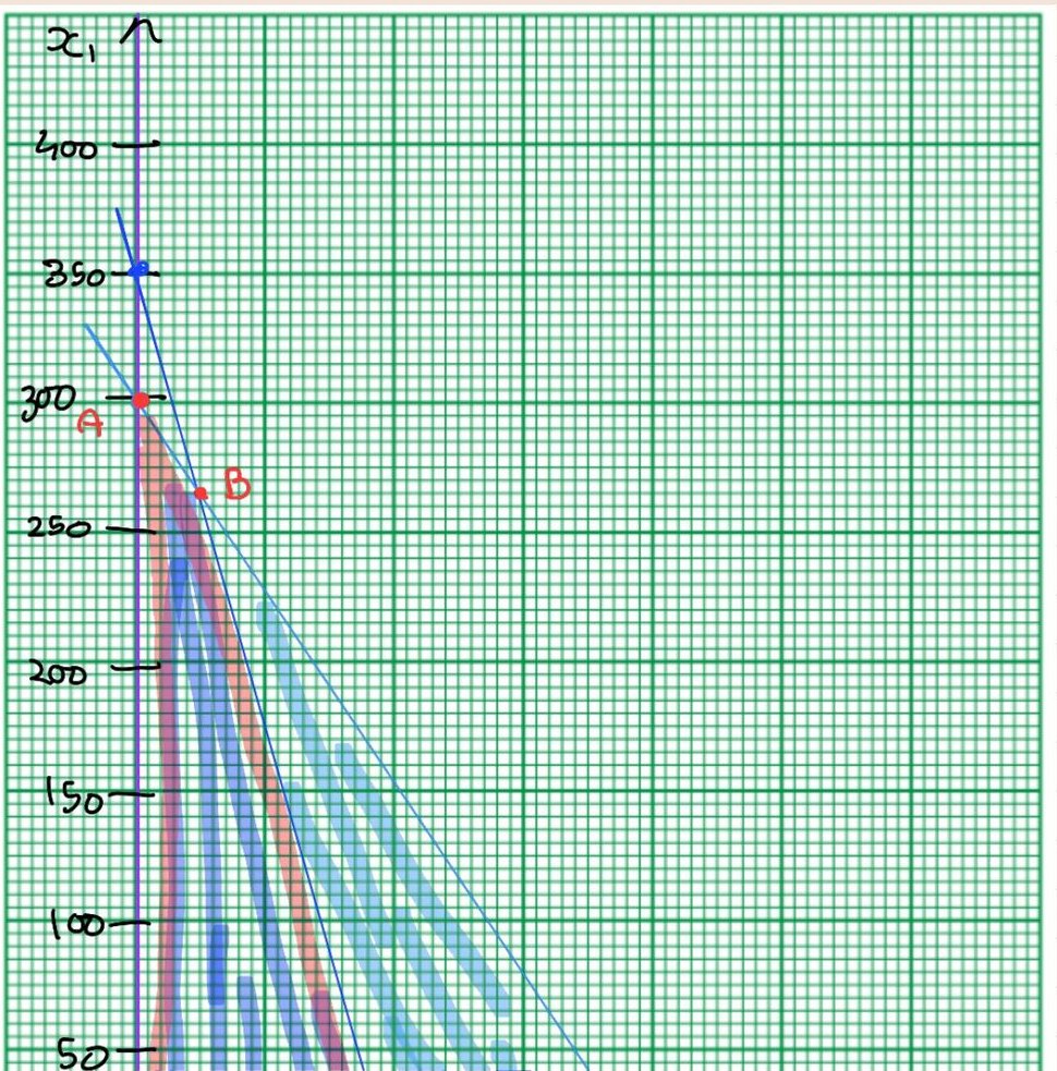
- Reading the intersection off the graph instead of solving it. Corner E is (25, 260), not "about (25, 260)". Solve the two equations simultaneously and show that working.
- Forgetting the origin. O(0,0) is a corner point of the feasible region whenever all constraints are ≤. Include it in the table.
- Shading the wrong side. Test the origin in each constraint: if (0,0) satisfies it, shade toward the origin. For a ≥ constraint it usually will not.
- Stopping at the corner point. The answer is the decision and the value of Z, with units — "25 tables and 260 chairs, profit ₹28,400".
Practice B1–B4 — 4 graphical problems with full corner-point tables →
4. The Five Special Cases Core syllabus concept
1Understand the Concept
Most LPPs have one clean optimum. Five things can go differently — and the exam asks you to recognise which one has happened from a tableau or a graph. Final Exam Q7A was exactly this, for 5 marks QP p. 5. Learn the identification signal for each; that is what is being marked.
| Case | What it means | Signal in the simplex tableau | Signal on the graph |
|---|---|---|---|
| 1. Unique optimum | Exactly one optimal solution. | All Cⱼ − Zⱼ < 0 for non-basic variables (Max problem). | Objective line touches the region at exactly one corner. |
| 2. Multiple optimal solutions | More than one combination gives the same best Z. Management gets a free choice. | A non-basic variable has Cⱼ − Zⱼ = 0 in the optimal table. | Objective line is parallel to a binding constraint — it touches along a whole edge. |
| 3. Unbounded solution | Z can grow infinitely. Always means the problem was formulated wrongly — no real business earns infinite profit. | No positive replacement ratio — all ratios are negative or infinite, so there is no outgoing variable. | Feasible region is open in the direction of improvement. |
| 4. Infeasible solution | No point satisfies all constraints at once. | An artificial variable stays in the basis at a non-zero value when the optimality condition is already met. | No common shaded region exists. |
| 5. Degenerate solution | A basic variable equals zero. Causes cycling risk. | At least one basic variable has value 0 in the Quantity column — caused by a tie in the replacement ratio. | Three or more constraints pass through the same corner point. |
2The class example for each case
All four are from the Special Cases deck pp. 1–7, and the infeasible one is reproduced in the class notes p. 19.
Degenerate = a basic variable is zero (look in the Quantity column). Multiple optima = a non-basic variable has Cⱼ − Zⱼ = 0 (look in the index row). Different column, different row, different diagnosis. Q7A of the Final paper turns exactly on telling them apart.
Practice D1–D4 — identify the case from four tableaux →
5. The Simplex Method Core syllabus concept
1Understand the Concept
The graphical method dies at three variables. The simplex method is an algebraic procedure that walks from one basic feasible solution (corner point) to a better adjacent one, and stops when no further improvement is possible.
2Step 1 — convert inequalities into equations
| Constraint type | Add | Meaning |
|---|---|---|
| ≤ | + Slack variable (S) | The unused amount of that resource. |
| ≥ | − Surplus variable, then + Artificial variable (A) | Surplus = the amount by which you exceed the requirement. The artificial variable only exists to give a starting basis. |
| = | + Artificial variable (A) | Again purely to start the algorithm. |
Setting X₁ = X₂ = 0 then gives the initial basic feasible solution: the slack variables equal the RHS values, and Z = 0 Notes p. 25.
3Step 2 — the tableau vocabulary
| Term | What it is |
|---|---|
| Cⱼ row | Objective coefficient of each variable. |
| Basic variables | The variables currently in the solution (non-zero). Listed down the left. |
| Quantity (Qty) column | The current values of the basic variables — and Z at the bottom. |
| Zⱼ row | For each column: Σ (C of basic variable × that column's entry in the row). |
| Cⱼ − Zⱼ (index row) | Net contribution per unit if that variable enters the solution. This row drives every decision. |
| Key/pivot column | The entering variable — most positive Cⱼ − Zⱼ (Max problem). |
| Replacement ratio | Qty ÷ corresponding pivot-column entry, computed for every row. |
| Key/pivot row | The leaving variable — smallest non-negative replacement ratio. |
| Pivot element | The number where the pivot row and pivot column intersect. |
4Step 3 — the iteration loop
- Build the initial table with slack variables as the starting basis.
- Compute Zⱼ for every column, then Cⱼ − Zⱼ.
- Optimality test: for a Max problem, stop when all Cⱼ − Zⱼ ≤ 0. For a Min problem, stop when all Cⱼ − Zⱼ ≥ 0.
- Entering variable = most positive Cⱼ − Zⱼ ⟹ that is the pivot column.
- Leaving variable = smallest non-negative replacement ratio (Qty ÷ pivot-column entry) ⟹ that is the pivot row.
- The intersection is the pivot element.
- New pivot row = Old pivot row ÷ pivot element.
- Every other new row = Old row − (that row's pivot-column entry × New pivot row).
- Recompute Zⱼ and Cⱼ − Zⱼ. Go back to step 3.
Full three-iteration worked example (Tables & Chairs) in the notes pp. 26–29, and step by step in the lecture deck pp. 19–25.
- Using a negative or zero replacement ratio. Only positive ratios are candidates. If none exist, the problem is unbounded — say so.
- Flipping the optimality test. Max stops at all Cⱼ − Zⱼ ≤ 0; Min stops at all Cⱼ − Zⱼ ≥ 0. Write which one you are doing at the top of the answer.
- Row operations on the pivot row last. Always compute the new pivot row first, then use it to update every other row.
Practice C1–C2 — two full simplex runs, every tableau shown →
6. Duality in Linear Programming Core syllabus concept
1Understand the Concept
Every LPP (the primal) has a mirror-image partner (the dual). If the primal asks "what production plan maximises profit given these resources?", the dual asks "what is each resource worth?" — and its optimal variable values are exactly the shadow prices of the primal. That is why duality and sensitivity analysis are taught together.
"Convert the given LPP primal to its dual" was Q1A in both the Final and the Re-Exam, worth 2.5 marks each time Final QP p. 1 Re-Exam QP p. 1. It is the single most predictable 2.5 marks available. Both versions solved step by step →
2The conversion procedure
| Step | Rule |
|---|---|
| 1. Canonical form first | For a Max primal, every constraint must be ≤. For a Min primal, every constraint must be ≥. Multiply a wrong-way inequality by −1 to flip it. Split every = constraint into two: one ≤ and one ≥ (then flip the ≥ one). |
| 2. Flip the objective | Max primal → Min dual. Min primal → Max dual. |
| 3. Swap roles | Primal with m constraints and n variables gives a dual with m variables (Y₁…Yₘ) and n constraints. |
| 4. Swap RHS and objective coefficients | The primal's RHS values (b) become the dual's objective coefficients; the primal's objective coefficients (c) become the dual's RHS. |
| 5. Transpose the matrix | Primal rows become dual columns. |
| 6. Flip the constraint direction | Max primal (≤) → dual constraints are ≥. Min primal (≥) → dual constraints are ≤. |
Both exam versions deliberately include an = constraint and a wrong-direction inequality. Here is the mechanical fix:
- An = constraint becomes two dual variables — one for the ≤ half and one for the ≥ half. They appear in the dual as +Y₃ − Y₄.
- A ≥ constraint in a Max primal must be multiplied by −1 to become ≤. Every coefficient and the RHS flip sign — which is why the synoptic answer has −10Y₂ and −2Y₂ terms.
- Count your dual variables before you start: number of primal constraints, with equalities counted twice. The Final's primal had 3 constraints (one of them =), so the dual has 4 variables — matching the key exactly Key p. 1.
3Quick reference — Primal ↔ Dual
| Primal (Max) | Dual (Min) |
|---|---|
| Maximise | Minimise |
| n variables | n constraints |
| m constraints | m variables |
| Objective coefficients (c) | RHS values |
| RHS values (b) | Objective coefficients |
| Constraints ≤ | Constraints ≥ |
| Coefficient matrix A | Transpose Aᵀ |
Practice E1–E5 — 5 primal→dual conversions, hardest last →
7. Sensitivity Analysis Core syllabus concept
1Understand the Concept
Sensitivity analysis — also called post-optimality analysis — studies the effect on the optimal solution of changes in the problem's parameters Deck p. 2. It answers two questions:
- How do changes in the objective function coefficients affect the optimal solution?
- How do changes in the right-hand-side values of the constraints affect it?
A "read this sensitivity report and answer five questions" item appeared in both papers — Final Q4A and Re-Exam Q4B Final p. 3 Re-Exam p. 3. You are never asked to produce the report, only to interpret it. Both solved →
2The four things a report tells you
| Term | Definition | How to use it in an answer |
|---|---|---|
| Reduced cost | How much the objective coefficient of a currently unused variable must improve before that variable enters the optimal solution. | Reduced cost = 0 ⟹ the variable is in the solution (it is basic, value > 0). Reduced cost ≠ 0 ⟹ the variable is not produced, and its profit must rise by that amount before it would be. |
| Objective coefficient range | Lower limit = current coefficient − allowable decrease; Upper limit = current coefficient + allowable increase. | As long as the coefficient stays inside the range, the optimal quantities do not change. Crucially — the optimal Z value does change. |
| Shadow price (dual value) | The improvement in the optimal objective value from a one-unit increase in that constraint's RHS, provided the change stays within the allowable range. | Change in Z = shadow price × change in RHS. Say it in money: "one extra hour of carpentry is worth ₹14.69 of extra profit". |
| Binding vs non-binding | A constraint is binding when it is fully used up. | Binding: slack/surplus = 0 and shadow price ≠ 0. Non-binding: slack/surplus ≠ 0 and shadow price = 0. Quote both numbers as your evidence. |
"Optimal solution does not change" does NOT mean "objective value does not change" Deck p. 9. If a profit coefficient moves inside its allowable range, you still produce the same quantities — but you earn a different profit. State both halves: "the optimal solution remains X₁ = 60, X₂ = 40, but Z changes to 45(60) + 20(40) = ₹3,500."
3The class worked example — advertising spaces
Optimal: X₁ = 60, X₂ = 40. Shadow price on square footage = 0.4.
| Question | Answer | Reasoning pattern |
|---|---|---|
| How much of the advertisement budget is spent? | 280 | Read the "used" value; the constraint is not fully consumed, so it is non-binding. |
| How much square footage is used? | 8000 | Fully consumed ⟹ binding ⟹ it has a non-zero shadow price. |
| Would the solution change if the budget became 300 instead of 400? | No | 300 lies in the allowable range (280 → ∞), so the basis holds. |
| What if profit on large space fell from 50 to 45? | Quantities unchanged; Z becomes ₹3,500 | 45 lies inside the range (40 → ∞). Then recompute: 45(60) + 20(40) = 3500. |
| How much do earnings rise if square footage goes 8000 → 9000? | +₹1,200 | Within range, so use the shadow price: 0.4 × 3000 = 1200. |
| Will the solution change if small-space profit goes 20 → 30? | Check against X₂'s allowable range | Same test as row 4 — compare the new coefficient with the printed bounds. |
| Will it change if large-space profit goes 50 → 35? | 35 is below the lower bound of 40 ⟹ yes, the basis changes | Outside the range ⟹ you can no longer say the solution holds; it must be re-solved. |
Questions and answers from the Sensitivity and Duality deck pp. 15–18; the class notes add the same interpretation in shorthand p. 1.
Practice F1–F4 — including a shadow price used beyond its range →