Solved Papers
Every Unit 1–3 question from the 2025-26 Final and Re-Examination, screenshotted from the original paper and worked in full — with the method, the arithmetic, and the way to lay the answer out on the page.
Each question shows the original screenshot from the paper, then a full solution, then a marks breakdown taken from the official synoptic answer key. Every solution here has been checked against that key — and where the key contains an arithmetic slip or an internal contradiction, it is flagged rather than copied.
Questions from Units 4–7 (game theory, queuing, simulation, decision theory, AHP) are not solved here — they are outside the Unit 1–3 portion your notes cover. They are listed in the Question Bank so you know they exist.
Final Q1A — Primal to Dual 2.5 marks · Unit 1
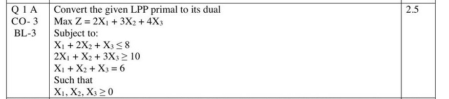
Step 1 — Convert to canonical form. The primal is a Max problem, so every constraint must become ≤.
| Original | Action | Canonical | Dual variable |
|---|---|---|---|
| X₁ + 2X₂ + X₃ ≤ 8 | Already ≤ | X₁ + 2X₂ + X₃ ≤ 8 | Y₁ |
| 2X₁ + X₂ + 3X₃ ≥ 10 | Multiply by −1 | −2X₁ − X₂ − 3X₃ ≤ −10 | Y₂ |
| X₁ + X₂ + X₃ = 6 | Split: the ≤ half | X₁ + X₂ + X₃ ≤ 6 | Y₃ |
| Split: the ≥ half, ×(−1) | −X₁ − X₂ − X₃ ≤ −6 | Y₄ |
Three printed constraints, but the equality splits into two — so the dual has four variables. Counting them before you start is the single best guard against losing this mark.
Step 2 — Set up the dual. Max primal → Min dual. The primal's RHS values (8, −10, 6, −6) become the dual's objective coefficients:
Step 3 — One dual constraint per primal variable, reading down each column of the canonical form. Max primal ⟹ dual constraints are ≥, with the primal objective coefficients as RHS.
| Primal variable | Column coefficients (Y₁, Y₂, Y₃, Y₄) | Dual constraint |
|---|---|---|
| X₁ | 1, −2, 1, −1 | Y₁ − 2Y₂ + Y₃ − Y₄ ≥ 2 |
| X₂ | 2, −1, 1, −1 | 2Y₁ − Y₂ + Y₃ − Y₄ ≥ 3 |
| X₃ | 1, −3, 1, −1 | Y₁ − 3Y₂ + Y₃ − Y₄ ≥ 4 |
Final answer — write exactly this:
✓ Matches the synoptic key exactly Key p. 1.
Re-Exam Q1A — Primal to Dual (Min version) 2.5 marks · Unit 1
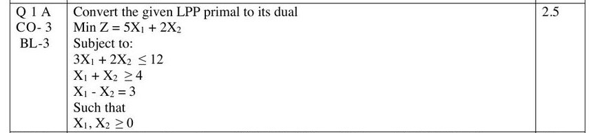
Step 1 — Canonical form. This one is a Min problem, so every constraint must become ≥ — the opposite direction to the Final's version.
| Original | Action | Canonical | Dual variable |
|---|---|---|---|
| 3X₁ + 2X₂ ≤ 12 | Multiply by −1 | −3X₁ − 2X₂ ≥ −12 | Y₁ |
| X₁ + X₂ ≥ 4 | Already ≥ | X₁ + X₂ ≥ 4 | Y₂ |
| X₁ − X₂ = 3 | Split: the ≥ half | X₁ − X₂ ≥ 3 | Y₃ |
| Split: the ≤ half, ×(−1) | −X₁ + X₂ ≥ −3 | Y₄ |
Step 2 — Dual objective. Min primal → Max dual, RHS values become the coefficients:
Step 3 — Dual constraints, one per primal variable, direction ≤:
| Primal variable | Column coefficients (Y₁, Y₂, Y₃, Y₄) | Dual constraint |
|---|---|---|
| X₁ | −3, 1, 1, −1 | −3Y₁ + Y₂ + Y₃ − Y₄ ≤ 5 |
| X₂ | −2, 1, −1, 1 | −2Y₁ + Y₂ − Y₃ + Y₄ ≤ 2 |
The printed key gives the first dual constraint as −3Y₁ + 2Y₂ + Y₃ − Y₄ ≤ 5 Key p. 1. But the coefficient of X₁ in the primal constraint X₁ + X₂ ≥ 4 is 1, not 2 — so the dual coefficient on Y₂ must be 1. The version above is the correct derivation. If you write +Y₂ you are right; the key slipped.
Final Q1B — Assignment: balanced? variables? constraints? 2.5 marks · Unit 3
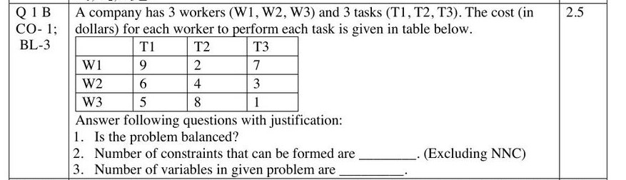
Identify the type first. There is no supply or demand row — every worker takes exactly one task. This is an assignment problem, m = 3 workers, n = 3 tasks.
| Sub-question | Answer | Justification to write |
|---|---|---|
| 1. Is the problem balanced? | Yes | For an assignment problem, balanced means number of rows = number of columns. Here 3 = 3, so it is balanced and no dummy is needed. |
| 2. Number of constraints (excluding NNC) | 6 | m + n = 3 + 3 = 6 — one constraint per worker (each does exactly one task) and one per task (each is done by exactly one worker). |
| 3. Number of variables | 9 | m × n = 3 × 3 = 9 — one binary variable Xᵢⱼ per cell of the cost matrix. |
✓ Matches the key: "Yes Problem is balanced as Number of rows = number of column; m+n = 6; mn = 9" Key p. 1.
Re-Exam Q1B — Transportation, and this one is unbalanced 2.5 marks · Unit 3
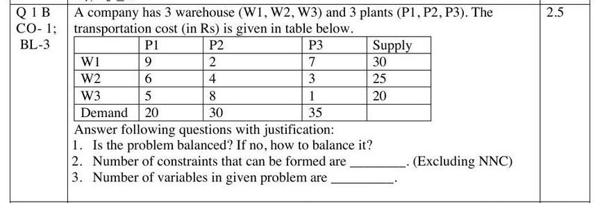
Identify the type. A supply column and a demand row are given ⟹ transportation problem.
Balance test — always compute both totals explicitly:
| Sub-question | Answer | Justification to write |
|---|---|---|
| 1. Balanced? If not, how to balance? | No. Add a dummy row (source) with supply = 10 and all costs = 0. | Balanced requires Σ supply = Σ demand. Demand is short by 10 on the supply side, so a dummy source supplies the missing 10 units at zero cost — those units are never actually shipped. |
| 2. Number of constraints (excluding NNC) | 6 | m + n = 3 + 3 = 6, counted on the original matrix. |
| 3. Number of variables | 9 | m × n = 3 × 3 = 9. |
✓ Matches the key Key p. 1, which also counts m + n and m × n on the original 3 × 3 matrix rather than the balanced 4 × 3 one.
Final Q3B — Formulate an LPP (chairs and tables) 5 marks · Unit 1

Step 0 — build the resource table. Do this before writing anything else:
| Resource | Per chair (X₁) | Per table (X₂) | Available |
|---|---|---|---|
| Carpentry (hours) | 4 | 3 | 120 |
| Finishing (hours) | 2 | 3 | 90 |
| Profit (₹/unit) | 200 | 300 | — maximise |
The question says "Formulate" — so stop here. No graph, no simplex.
| Component | Marks |
|---|---|
| Correctly defining variables | 1 |
| Objective function formed properly | 1 |
| Two constraints formulated accurately | 2 |
| Non-negativity stated | 1 |
Read that breakdown carefully. Defining the variables and stating non-negativity are worth 2 of the 5 marks — two lines that take ten seconds. Never skip them.
Re-Exam Q3B — Formulate an LPP (two products, two raw materials) 5 marks · Unit 1

| Resource | Per P1 (X₁) | Per P2 (X₂) | Available |
|---|---|---|---|
| Raw material A | 5 | 3 | 150 |
| Raw material B | 3 | 6 | 180 |
| Profit (₹/unit) | 40 | 50 | — maximise |
✓ Matches the key exactly Key p. 3, including the same 1 / 1 / 2 / 1 mark split.
Final Q4A — Interpret the sensitivity report 5 marks · Unit 1
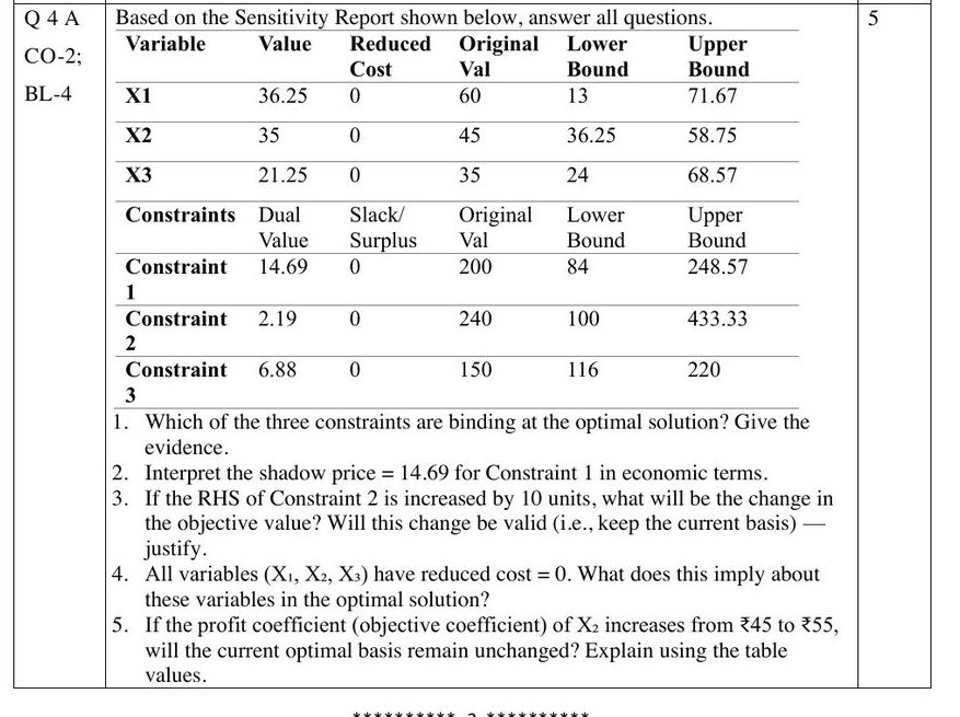
(1) Which constraints are binding? Give the evidence.
All three are binding. The test has two halves and you should quote both:
| Constraint | Slack / Surplus | Dual value | Verdict |
|---|---|---|---|
| Constraint 1 | 0 | 14.69 | Binding |
| Constraint 2 | 0 | 2.19 | Binding |
| Constraint 3 | 0 | 6.88 | Binding |
Zero slack means the resource is fully consumed; a non-zero shadow price means more of it would still be worth something. Both conditions hold for all three, so every resource is a genuine bottleneck.
(2) Interpret the shadow price 14.69 for Constraint 1 in economic terms.
(3) If the RHS of Constraint 2 increases by 10 units, what is the change in objective value? Is it valid?
Because the change is within range, the shadow price is still the right multiplier and the same variables remain basic.
(4) All variables have reduced cost = 0. What does that imply?
All three variables are basic — they are in the optimal solution at positive levels (X₁ = 36.25, X₂ = 35, X₃ = 21.25). A reduced cost of zero means no improvement to that variable's objective coefficient is needed to justify producing it; it is already worth producing.
A reduced cost of 0 on a non-basic variable would signal alternate optimal solutions. That is not the case here, because all three variables have non-zero values and so are basic. Saying that sentence out loud earns the mark Key p. 4.
(5) If the coefficient of X₂ rises from ₹45 to ₹55, does the basis stay optimal?
But the objective value does change. Add this line to separate a good answer from a full one:
Re-Exam Q4B — Sensitivity report with a non-binding constraint 5 marks · Unit 1
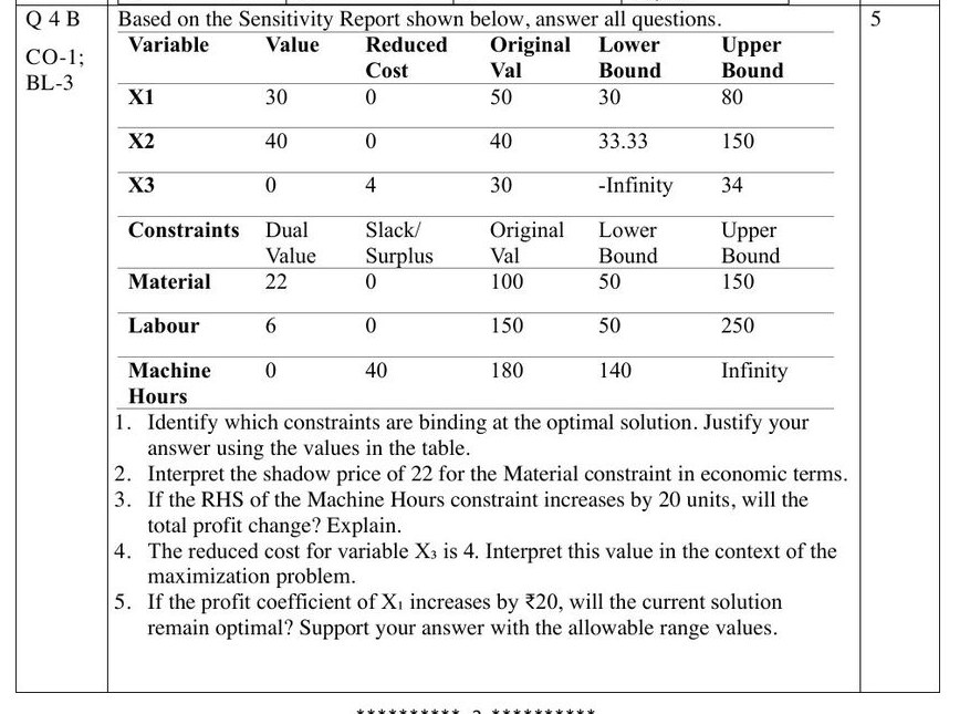
(1) Which constraints are binding?
| Constraint | Slack / Surplus | Dual value | Verdict |
|---|---|---|---|
| Material | 0 | 22 | Binding |
| Labour | 0 | 6 | Binding |
| Machine Hours | 40 | 0 | NOT binding |
Material and Labour are binding — slack = 0 and shadow price > 0. Machine Hours is not: it has 40 units of unused capacity and a shadow price of 0, so it is not limiting the solution at all.
(2) Interpret the shadow price of 22 for Material.
(3) If Machine Hours RHS increases by 20 units, will profit change?
No — profit is unchanged. Two reasons, both worth stating: the shadow price is 0, so ΔZ = 0 × 20 = 0; and there are already 40 unused machine hours. Adding more of a resource you are not fully using cannot help. Machine Hours is a non-binding constraint.
(4) The reduced cost of X₃ is 4 — interpret it.
X₃ has value 0: it is not produced in the optimal solution. The reduced cost of 4 can be stated two equivalent ways, and either earns the mark:
- Forcing one unit of X₃ into the solution would reduce total profit by ₹4.
- Equivalently, X₃'s profit coefficient would have to rise by ₹4 — from ₹30 to ₹34 — before it becomes worth producing.
Notice the internal check: X₃'s upper bound in the table is 34 = 30 + 4. The report is consistent with itself, and quoting that agreement is a strong touch.
(5) If the profit coefficient of X₁ increases by ₹20, does the solution stay optimal?
Quantities stay X₁ = 30, X₂ = 40, X₃ = 0, but profit rises:
Final Q4B — Formulate an ILP (Maverick Analytics) 5 marks · Unit 2
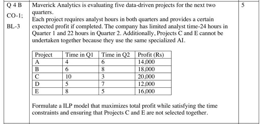
Step 1 — spot the variable type. "Which projects should be undertaken" ⟹ each project is a yes/no decision ⟹ binary variables, not quantities.
Step 2 — objective function. Maximise total expected profit:
Step 3 — resource constraints. One per quarter, read straight down the table columns:
Step 4 — the logical constraint. This is the sentence buried at the end of the stem: "Projects C and E cannot be undertaken together."
Step 5 — the binary condition. Without this line the model is an LP, not an ILP:
| Component | Marks |
|---|---|
| Identification of decision variables | 1 |
| Formulation of objective function | 1 |
| Formulation of constraints | 2 |
| Binary condition + overall clarity of model structure | 1 |
The binary condition is a full mark on its own. Write it as its own labelled line.
Re-Exam Q4A — Formulate an ILP (Orion Tech Services) 5 marks · Unit 2
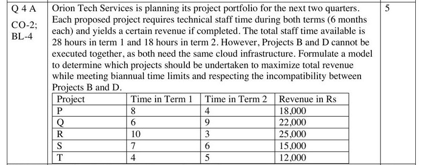
The stem says "Projects B and D cannot be executed together", but the table lists projects P, Q, R, S, T — there is no B or D. This is leftover wording from the Final paper's version (which did have projects A–E). The defensible reading is that B and D mean the second and fourth projects in the table, i.e. Q and S. State that assumption in one line — the paper's own instruction 7 says "Assume suitable data if necessary", so you are explicitly permitted to.
The synoptic key prints its Q4A answer as an image with no extractable text Key p. 3, but its published mark split is identical to the Final's: variables 1, objective 1, constraints 2, binary condition 1.
Final Q5B — Formulate an assignment problem (flight scheduling) 5 marks · Unit 3
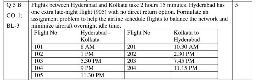
Step 1 — work out when each outbound flight lands. Flight time is 2 hours 15 minutes.
| Flight (Hyd → Kol) | Departs | Arrives Kolkata |
|---|---|---|
| 101 | 8:00 AM | 10:15 AM |
| 102 | 1:00 PM | 3:15 PM |
| 103 | 5:30 PM | 7:45 PM |
| 104 | 9:00 PM | 11:15 PM |
| 105 | 11:30 PM | 1:45 AM (next day) |
Step 2 — build the idle-time (cost) matrix. Idle time = return departure − arrival, rolling to the next day whenever the return leaves before the aircraft lands.
| Arrives ↓ / Returns → | 201 (10:30) | 202 (14:30) | 203 (19:45) | 204 (23:15) |
|---|---|---|---|---|
| 101 (10:15) | 0.25 | 4.25 | 9.5 | 13 |
| 102 (15:15) | 19.25 | 23.25 | 4.5 | 8 |
| 103 (19:45) | 14.75 | 18.75 | 24 | 3.5 |
| 104 (23:15) | 11.25 | 15.25 | 20.5 | 24 |
| 105 (01:45) | 8.75 | 12.75 | 18 | 21.5 |
Sample working: flight 102 lands at 15:15; return 203 leaves at 19:45; idle = 19:45 − 15:15 = 4 h 30 m = 4.5. Flight 104 lands 23:15; return 202 leaves 14:30 the next day; idle = 15 h 15 m = 15.25.
Step 3 — balance the problem. There are 5 outbound flights but only 4 returns — the stem tells you flight 105 has no direct return option. So:
Step 4 — write the assignment LPP.
The key prints two idle-time tables that disagree with each other Key p. 5. Checked against the timetable, the correct values are the ones above; the key's errors are:
- Cell 102 → 203: key says 4.25. Arrival 15:15, departure 19:45 ⟹ 4.5.
- Cell 104 → 202: key's two tables say 14.25 and 3.25. Arrival 23:15, departure 14:30 next day ⟹ 15.25.
Re-Exam Q5B — Assignment with a turnaround requirement 5 marks · Unit 3
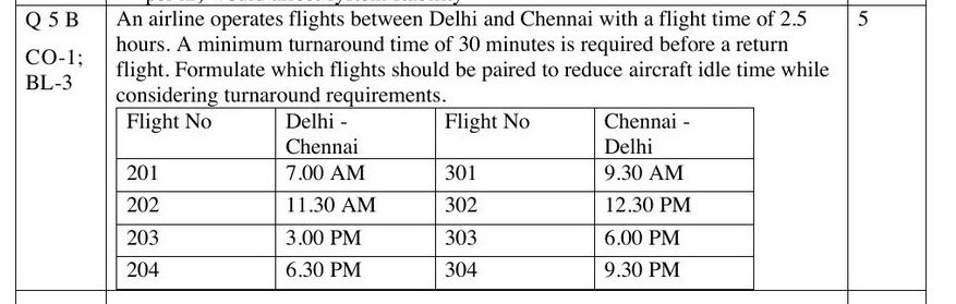
Step 1 — arrival times. Flight time 2.5 hours.
| Flight (Del → Che) | Departs | Arrives Chennai |
|---|---|---|
| 201 | 7:00 AM | 9:30 AM |
| 202 | 11:30 AM | 2:00 PM |
| 203 | 3:00 PM | 5:30 PM |
| 204 | 6:30 PM | 9:00 PM |
Step 2 — idle time, net of the 30-minute turnaround. This is what makes this version harder than the Final's. A pairing is only feasible if the gap is more than the 30-minute turnaround; otherwise the aircraft must wait until the same flight the next day. The cost recorded is the idle time beyond the required turnaround, i.e. gap − 0.5.
| Arrives ↓ / Returns → | 301 (9:30) | 302 (12:30) | 303 (18:00) | 304 (21:30) |
|---|---|---|---|---|
| 201 (9:30) | 23.5 | 2.5 | 8 | 11.5 |
| 202 (14:00) | 19 | 22 | 3.5 | 7 |
| 203 (17:30) | 15.5 | 18.5 | 24 | 3.5 |
| 204 (21:00) | 12 | 15 | 20.5 | 24 |
Sample working: 202 lands 14:00, return 303 departs 18:00 ⟹ gap 4 h, minus the 0.5 h turnaround = 3.5. Where the gap is only 0.5 h — 201→301 and 203→303 and 204→304 — the turnaround exactly consumes it, so the key rolls the aircraft to the same service next day, giving 24. ✓ Every cell above matches the key Key p. 5.
Step 3 — the formulation. Here it is 4 × 4, already balanced — no dummy needed.
Final Q7A — Identify the special case from the final tableau 5 marks · Unit 1
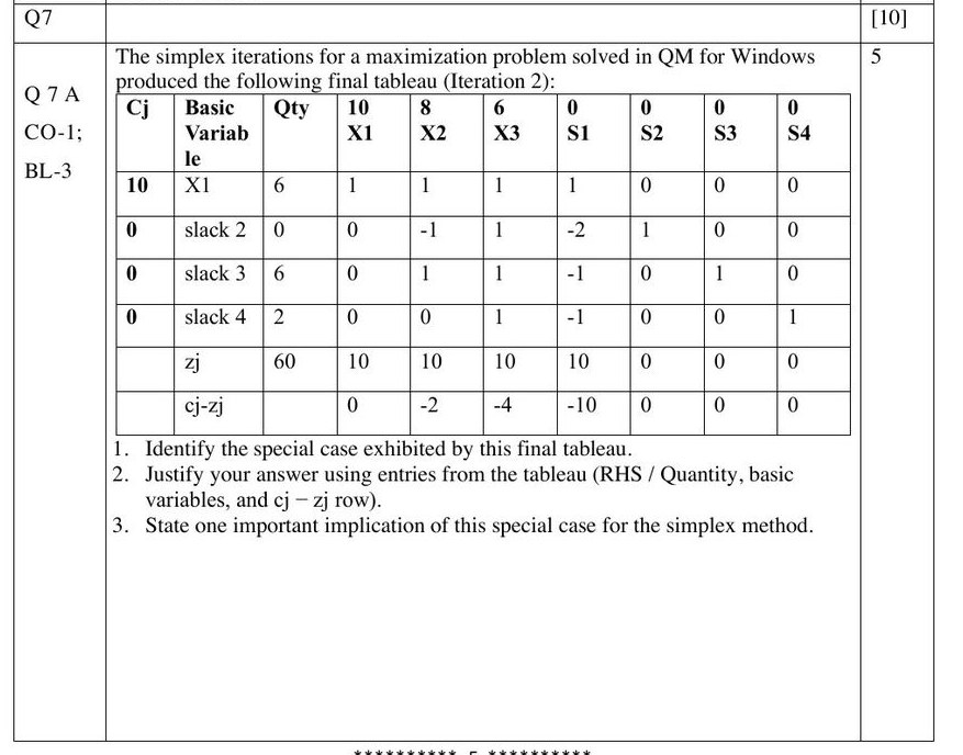
(1) The special case is DEGENERACY.
(2) Justification — three observations, each pointing at a specific part of the tableau:
| Where to look | What you see | What it proves |
|---|---|---|
| Quantity (RHS) column | slack 2 is a basic variable with Quantity = 0 |
A basic variable at zero level is the definition of a degenerate basic feasible solution. |
| Cⱼ − Zⱼ row | All values ≤ 0 (0, −2, −4, −10, 0, 0, 0) | For a maximisation problem this is the optimality condition — so the tableau is already optimal. Hence degeneracy at optimality. |
| Cⱼ − Zⱼ, non-basic columns | X₂ = −2, X₃ = −4, S₁ = −10 — all strictly negative | Rules out multiple optimal solutions, which would need a non-basic variable at exactly 0. This is the distinction the question is testing. |
(3) One important implication for the simplex method:
✓ Matches the key's three-part structure — identification, justification, implication — almost word for word Key p. 7.
Under time pressure it is easy to see "a zero in the Cⱼ − Zⱼ row" and answer multiple optima. But those zeros sit in the basic columns (X₁, S₂, S₃, S₄), where a zero is expected and means nothing. The zero that matters for multiple optima must be on a non-basic variable. Here the zero that matters is in the Quantity column instead — different row, different diagnosis.
Final Q7B — Transportation format with a profit twist 5 marks · Unit 3
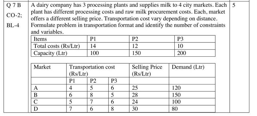
Step 1 — spot the twist. This is not a plain cost-minimisation. You are given plant costs, transportation costs and selling prices — so the cell value must be a profit, and the objective becomes Max.
Step 2 — build the profit matrix. Compute cell by cell:
| Cell | Working | Profit |
|---|---|---|
| P1 → A | 25 − 14 − 4 | 7 |
| P2 → A | 25 − 12 − 5 | 8 |
| P3 → A | 25 − 10 − 6 | 9 |
| P1 → B | 28 − 14 − 6 | 8 |
| P2 → B | 28 − 12 − 8 | 8 |
| P3 → B | 28 − 10 − 5 | 13 |
| P1 → C | 24 − 14 − 5 | 5 |
| P2 → C | 24 − 12 − 7 | 5 |
| P3 → C | 24 − 10 − 6 | 8 |
| P1 → D | 30 − 14 − 7 | 9 |
| P2 → D | 30 − 12 − 6 | 12 |
| P3 → D | 30 − 10 − 8 | 12 |
Step 3 — lay it out in transportation format.
| Plant | A | B | C | D | Supply |
|---|---|---|---|---|---|
| P1 | 7 | 8 | 5 | 9 | 100 |
| P2 | 8 | 8 | 5 | 12 | 150 |
| P3 | 9 | 13 | 8 | 12 | 200 |
| Demand | 120 | 150 | 100 | 80 | 450 / 450 |
✓ This profit matrix matches the synoptic key cell for cell Key p. 8.
Step 4 — balance check and the counts the question asks for.
Step 5 — the LPP.
Seven constraints — exactly the m + n you computed. Because supply and demand are perfectly balanced, the supply constraints may be written as = rather than ≤.
| Slot | What it always is | Unit | Marks |
|---|---|---|---|
| Q1A | Primal → Dual conversion, always with one = and one wrong-way constraint | 1 | 2.5 |
| Q1B | Cost matrix → balanced? · m + n · m × n | 3 | 2.5 |
| Q3B | Formulate an LPP from a two-product, two-resource story | 1 | 5 |
| Q4 (one part) | Interpret a sensitivity report — 5 sub-questions | 1 | 5 |
| Q4 (other part) | Formulate an ILP — project selection + one logical constraint | 2 | 5 |
| Q5B | Flight-pairing assignment problem | 3 | 5 |
| Q7A | Identify the special case from a final simplex tableau | 1 | 5 |
| Q7B | Transportation formulation, often with a profit twist | 3 | 5 |
That is 35 marks of the 50 available, all from Units 1–3. Q1 is compulsory and you choose 4 of the remaining 6 — so a candidate who is fluent in these eight patterns can build a complete paper without touching game theory, queuing, simulation or decision theory.