Unit 10 — Job Sequencing and Scheduling
Deciding what work goes where, in what order, and how to track it once it's running.
1. Production Planning & Control: Loading, Sequencing, Monitoring Core syllabus concept
1Understand the Concept
Scheduling is the last stage of planning before production actually happens — it specifies exactly when labour, equipment, and facilities will be used to produce a job. In a job shop, where a wide variety of jobs with different routings compete for the same limited resources at any given time, scheduling is genuinely difficult, and is carried out by a production control department. This function is also known as shop floor control (SFC), and it breaks down into three distinct responsibilities that map exactly onto your syllabus's three named topics:
- Loading — checking the availability of material, machines, and labour, and assigning work to specific resources.
- Sequencing — releasing work orders to the shop floor and deciding, when several jobs compete for one resource, which one gets processed first.
- Monitoring — tracking the progress of each job until completion, and reporting on it (since plans often need to be revised as the shop floor situation changes).
Scheduling objectives are often in conflict with one another — meeting due dates, minimising lateness, minimising completion time, maximising machine/labour utilisation, and minimising work-in-process inventory can all pull in different directions, which is exactly why the specific sequencing rules covered later in this unit exist: different rules optimise for different objectives.
2Simple Explanation
3Important Points
- Scheduling = the last planning stage before production; particularly complex for job-shop (batch) production due to job variety and resource competition.
- Also called shop floor control (SFC), production control, or production activity control (PAC).
- Three functions: Loading, Sequencing, Monitoring — detailed individually in the rest of this unit.
- Common scheduling objectives (often conflicting): meet due dates, minimise lateness/completion time/WIP, maximise utilisation.
4Exam-Ready Answer
Scheduling is the final stage of production planning, specifying when labour, equipment, and facilities are needed to complete a job, and is especially challenging in job-shop or batch production because a wide variety of jobs with different processing requirements compete simultaneously for limited resources. The production control department, also referred to as shop floor control, performs three linked functions. Loading involves checking the availability of material, machines, and labour, and assigning specific jobs to specific resources. Sequencing determines the order in which multiple jobs waiting at the same resource should be processed, typically guided by a sequencing rule. Monitoring tracks the progress of each job through the system, using tools such as Gantt charts, and generates reports that allow schedules to be revised as conditions on the shop floor change. Because scheduling objectives such as meeting due dates, minimising work-in-process, and maximising resource utilisation often conflict with one another, no single approach optimises every objective simultaneously, which is why different loading and sequencing techniques exist for different priorities.
5Possible Exam Questions
- Explain the functions of production planning and control with respect to scheduling.
- What is shop floor control? Name its three main functions.
- Why is scheduling more complex in a job shop than on an assembly line?
6Common Mistakes
- Treating loading, sequencing, and monitoring as interchangeable — each answers a distinct question (which resource / what order / how is it progressing).
2. Loading & the Assignment Method Core syllabus concept
1Concept — What Is It Solving?
Loading is the process of assigning work to limited resources — deciding which worker or machine handles which job. When several workers/machines could each do several jobs, but at different speeds or costs, the assignment method (a specialised linear-programming technique) finds the one-to-one pairing of jobs to resources that minimises total time or cost.
2Step-by-Step Method
- Row reduction: subtract the smallest value in each row from every value in that row.
- Column reduction: subtract the smallest value in each column (of the row-reduced table) from every value in that column.
- The result is an opportunity-cost matrix. Cover all zeros using the minimum number of horizontal/vertical lines.
- If the number of lines equals the number of rows, an optimal assignment exists at the zeros — assign accordingly. If not, subtract the smallest uncovered value from all uncovered values, and add it to every value where two lines intersect; then repeat step 3.
For a maximisation problem (e.g. maximising profit rather than minimising cost/time), first subtract every value in the original matrix from the largest value in the matrix, then proceed exactly as above.
3When to Use It
Use the assignment method whenever you must pair up N jobs with N resources (workers, machines) one-to-one, given a table of times/costs for every possible job-resource pairing, and you want the pairing that minimises total time or cost (or maximises total profit/output).
4Textbook Example — Example 17.1
WebStar Inc. has 4 workers and 4 projects, with estimated hours for each worker-project pair:
| Project 1 | Project 2 | Project 3 | Project 4 | |
|---|---|---|---|---|
| Bryan | 10 | 5 | 6 | 10 |
| Kari | 6 | 2 | 4 | 6 |
| Noah | 7 | 6 | 5 | 6 |
| Chris | 9 | 5 | 4 | 10 |
After row reduction, column reduction, and one round of matrix adjustment (since the first covering needed only 3 lines for a 4×4 table), the optimal assignment is: Bryan → Project 2, Kari → Project 1, Noah → Project 4, Chris → Project 3.
Total time = 5+6+6+4 = 21 hours. At $100/hour, minimum total cost = $2,100.
5Important Points
- Assignment method = a specialised linear-programming procedure; strictly one-to-one pairing (each worker/machine gets exactly one job).
- For minimisation: row reduction → column reduction → cover zeros → adjust if needed → assign.
- For maximisation: convert to a minimisation problem first by subtracting every entry from the matrix's largest value.
- Verify the final assignment against the original matrix (not the reduced one) to compute actual total time/cost.
6Common Mistakes
- Forgetting to convert a maximisation problem into minimisation form before applying the method.
- Reading off the final total cost from the reduced matrix instead of the original matrix.
- Stopping after row+column reduction without checking whether the minimum number of covering lines actually equals the matrix size.
3. Sequencing Rules for One Process Core syllabus concept
1Concept — What Is It Solving?
Once jobs are loaded onto a resource, sequencing decides the order in which they are processed. When several jobs queue at one machine, a sequencing rule is needed — and different rules optimise for different objectives, so there is no single rule that is best on every measure at once.
2The Rules
- FCFS (first-come, first-served) — process jobs in arrival order.
- DDATE (earliest due date) — process the job due soonest, first.
- SPT (shortest processing time) — process the quickest job first.
- LPT (longest processing time) — process the longest job first.
- SLACK — process the job with least slack first, where Slack = (due date − today's date) − remaining processing time.
- CR (critical ratio) — CR = (due date − today's date) / remaining processing time. CR > 1 = ahead of schedule; CR < 1 = behind schedule; CR = 1 = exactly on schedule.
3When to Use Which Rule
- SPT is best when the shop is highly congested — it minimises mean flow time and the number of jobs in the system (WIP), but risks a few long jobs becoming very late.
- SLACK works well for periods of normal activity, balancing due date and processing time together.
- DDATE is best when only small tardiness can be tolerated — it minimises mean and maximum tardiness.
- LPT suits situations where subcontracting is anticipated, so large jobs are finished in-house and small ones can be sent out.
- FCFS is simplest and works fine when the shop is operating well below capacity.
4Textbook Example — Example 17.2
5 jobs (A–E) with given processing times and due dates are sequenced four different ways. Summary of results:
| Rule | Avg. Completion Time | Avg. Tardiness |
|---|---|---|
| FCFS | 18.60 | 9.6 |
| DDATE | 15.00 | 5.6 (best) |
| SLACK | 16.40 | 6.8 |
| SPT | 14.80 (best) | 6.0 |
This confirms the theory: SPT minimises average completion (flow) time, while DDATE minimises average tardiness — no single rule wins on both measures simultaneously.
5Important Points
- Flow time = time for a job to be completed from when it entered the queue; makespan = total time to finish a whole group of jobs (does not change no matter the sequence, for a single machine); tardiness = (completion time − due date), if positive.
- No sequencing rule optimises both processing efficiency (flow time) and due-date performance (tardiness) simultaneously — this is provable, not just observed.
- SPT provably minimises mean flow time and mean number of jobs in the system; DDATE minimises mean tardiness.
6Common Mistakes
- Computing tardiness as (due date − completion time) instead of (completion time − due date); tardiness cannot be negative — an early job has zero tardiness, not negative tardiness.
- Forgetting that the start time of each job equals the completion time of the previous job in sequence.
- Assuming makespan changes with sequence on a single machine — for one process it does not; only individual completion times and tardiness change.
4. Johnson's Rule (Two-Process Sequencing) Core syllabus concept
1Concept — What Is It Solving?
The rules above sequence jobs through a single process. Johnson's Rule, explicitly named in your syllabus, finds the sequence that minimises total completion time (makespan) when a set of jobs must pass through two processes in series, in the same order (e.g. every job goes through Process 1, then Process 2).
2Step-by-Step Method
- List the processing time for every job at both processes.
- Find the single smallest processing time anywhere in the whole table.
- If that smallest time is at Process 1, place that job as early as possible in the sequence. If it's at Process 2, place that job as late as possible in the sequence.
- Remove that job from consideration, and repeat steps 2–3 with the remaining jobs, filling in from both ends toward the middle until every job is placed.
3Textbook Example — Example 17.3
5 jobs (carousel animals) need sanding (Process 1) then painting (Process 2):
| Job | Process 1 | Process 2 |
|---|---|---|
| A | 6 | 8 |
| B | 11 | 6 |
| C | 7 | 3 |
| D | 9 | 7 |
| E | 5 | 10 |
Smallest time overall = 3 (Job C, Process 2) → place C last. Next smallest = 5 (Job E, Process 1) → place E first. Next = 6, tied between Job A (Process 1) and Job B (Process 2) → place A early, B late. Job D fills the only remaining (middle) slot.
Optimal sequence: E → A → D → B → C. Using this sequence to build a Gantt chart of both processes (a job cannot start Process 2 until it finishes Process 1, and Process 2 can only handle one job at a time), the total completion time (makespan) for all 5 jobs is 41 hours — faster than any other sequence.
4Important Points
- Johnson's Rule requires: every job follows the same two-process sequence (Process 1 then Process 2).
- It minimises makespan (total completion time) and idle time — it does not consider due dates, so it does not necessarily minimise tardiness.
- It's essentially a variation of SPT applied simultaneously at both ends of the sequence.
- The resulting sequence is identical at both processes (a job that goes 3rd at Process 1 also goes 3rd at Process 2).
5Common Mistakes
- Placing a Process-2 minimum job early instead of late (or vice versa) — remember: Process 1 minimum → front; Process 2 minimum → back.
- Forgetting that a job can't start Process 2 until it has finished Process 1, when constructing the Gantt chart/makespan.
- Applying Johnson's Rule to jobs that don't all follow the same two-process order — the rule assumes a strictly identical routing for every job.
5. Monitoring: Gantt Charts & Input/Output Control Core syllabus concept
1Understand the Concept
Once jobs are loaded and sequenced, production control must monitor their actual progress, since queues, machine breakdowns, and quality issues can all delay a job after it starts. Shop paperwork called a work package travels with each job, and workers sign off on it (or scan a barcode/RFID tag) as work is completed at each stage, feeding progress data back into the monitoring system.
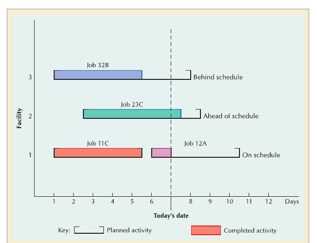
A Gantt chart is the classic tool for this: it displays both planned and actually-completed activity against a time scale, so a manager can see at a glance whether each job is ahead of, on, or behind schedule. Input/output (I/O) control is a complementary technique that monitors both the input to and output from each work centre — comparing only output against the plan (the older approach) can be misleading in an interconnected job shop, because low output at one centre might actually be caused by a shortage of input from an earlier centre, not a problem at the centre itself.
2Simple Explanation
3Example
4Important Points
- Gantt chart: shows planned vs. completed activity against time; instantly reveals whether a job is ahead, on, or behind schedule.
- Work package: shop paperwork travelling with the job, signed off (or scanned) at each stage.
- Input/output control: tracks both inflow and outflow at each work centre, to correctly diagnose whether a slowdown originates locally or upstream.
- Progress reports, exception reports (highlighting problems), and "hot lists" (highest-priority jobs) are all outputs of the monitoring function.
5Exam-Ready Answer
Monitoring is the function of tracking a job's progress through the shop floor and reporting on it so that schedules can be adjusted as conditions change. Shop paperwork known as a work package travels with each job and is signed off, manually or electronically, as work is completed at each stage. A Gantt chart is the most common monitoring tool, displaying both planned and actually completed activity against a time scale, which allows a manager to see at a glance whether a job is ahead of, exactly on, or behind schedule. Input/output control complements this by tracking both the input to and the output from each work centre, rather than output alone, since in an interconnected job shop a shortfall in output at one centre may actually be caused by insufficient input arriving from an earlier centre rather than a problem at that centre itself. Together, these tools allow production control to generate progress reports, exception reports, and priority ("hot") lists that keep the schedule realistic as the shop floor situation evolves.
6Possible Exam Questions
- Explain the role of Gantt charts in monitoring production schedules.
- What is input/output control, and why is it more informative than monitoring output alone?
- Interpret a given Gantt chart to identify which jobs are ahead of, on, or behind schedule.
7Common Mistakes
- Describing a Gantt chart as only a planning tool — in this unit's context, its key role is as a monitoring tool, comparing plan against actual progress.